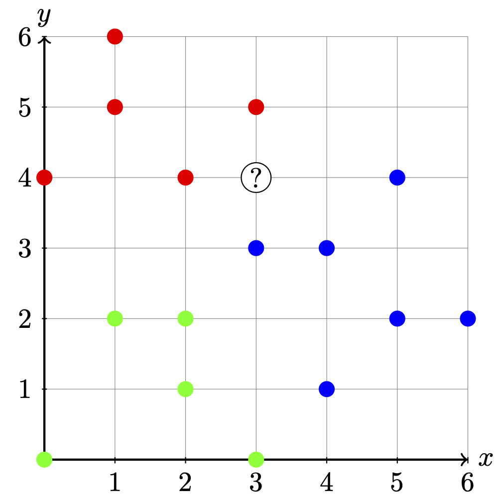
So far we have seen how we can predict quantitative outcomes using linear regression and classify binary outcomes using logistic regression, but what happens if we have multiple possible qualitative outcomes? To answer this question, we might try to classify a value by looking at what the other “similar” values are near it. The idea of identifying the closest \(k\) observations and predicting our outcome based on which values occur most is called KNN (K-Nearest Neighbors). If a tie occurs we randomly classify it. To get an idea of this, we can look at the following plot and try to predict what value the point \((3,4)\) would be:
9.1 The KNN Algorithm
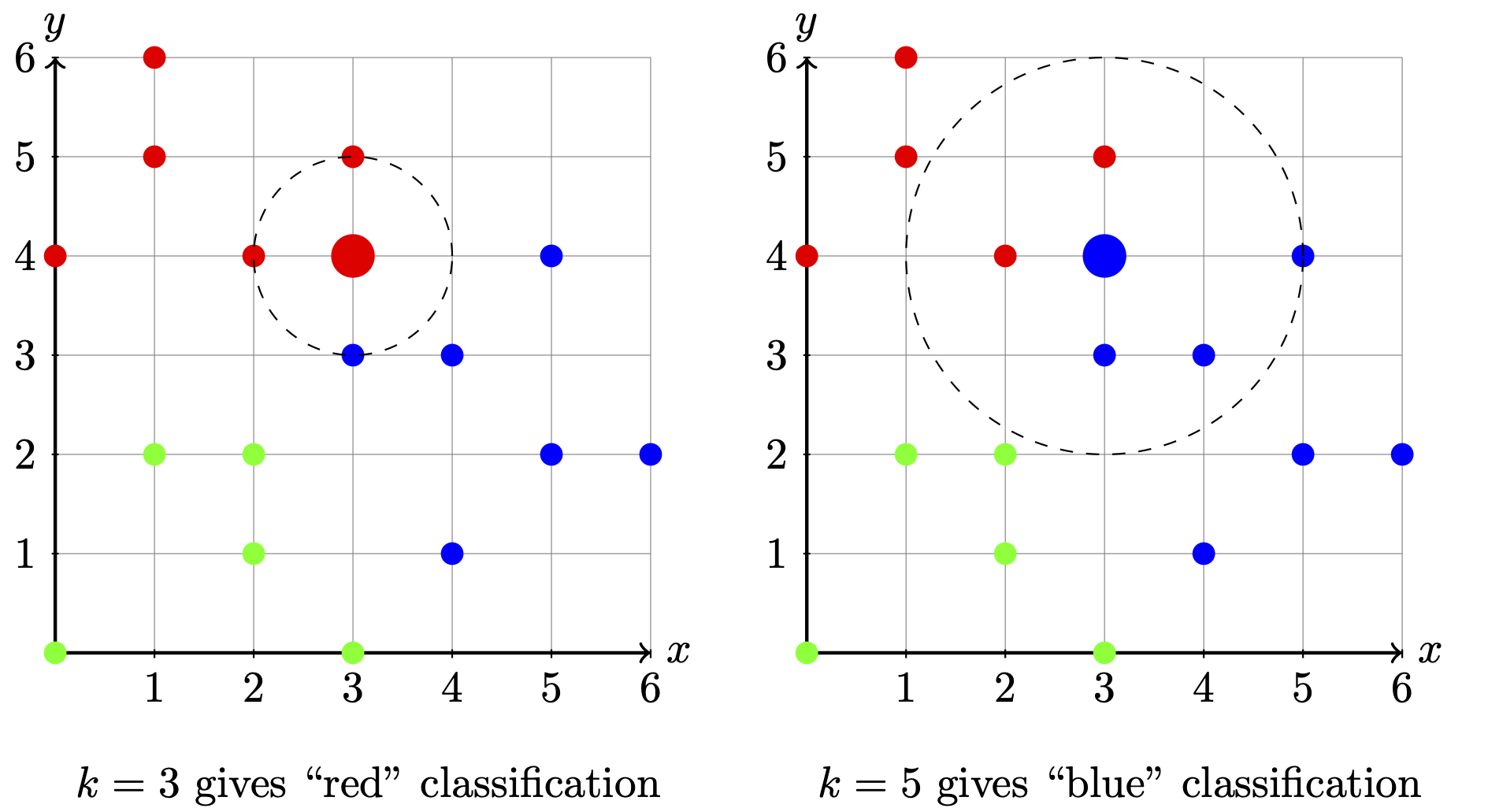
In order to predict what category the point \((3,4)\) would be, we would first need to identify the closest \(k\) points. We can define “close” in this case using the Euclidean distance formula \[d_i=\sqrt{(x_2 - x_1)^2 + (y_2 - y_1)^2}\] If we were to select the closest \(3\) observations then we would classify the point \((3,4)\) as “red”, but if we were to select the closest \(5\) observations then we would classify the point \((3,4)\) as “blue”. We can see that with the visualization below:
9.2 Measuring Similarity
We should note that were are multiple ways to define distance (and each may give us slightly different results!). The distance metric that we are probably most familiar with is the Euclidean distance (the straight line distance between 2 points) defined as \[d_i=\sqrt{(x_2 - x_1)^2 + (y_2 - y_1)^2}\] The Manhattan distance (the “city blocks” distance between 2 points) can be defined as \[
d_i = |x_2 - x_1| + |y_2 - y_1|\] Other distance metrics that could be used to determine the similarity between values are the Cosine Distance, the Mahalanobis Distance, and the Chebyshev distance. Also, note that these distance metrics can be extended into higher dimensions.
If we had categorical predictors then we could also calculate which observations are the “most similar”. To do this, we will introduce the idea of the Jaccard distance and the Hamming distance. The Jaccard distance is interested in determining the proportion of features in common and can be calculated as \(J(A,B)=\frac{|A\cap B|}{|A \cup B|}\). We will typically define values “similar” to each other using the Jaccard dissimilarity (\(1-J(A,B)\)). The Hamming distance focuses on if the individual positions are different and increments by 1 if they are different. We will then look at the \(k\) most similar observations to determine what the new observation would be classified as. An example of this can be seen below:
9.3 Building a KNN Model in R
The KNN model can be run in R using the knn() function located within the class library. We will pass both the training and testing data into the function and it will automatically classify the values for us.
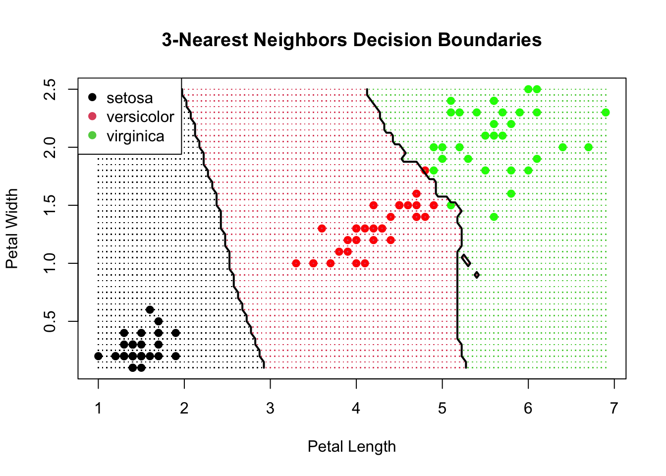
We can see from the results above that this model does fairly well in classifying the species, with only 4 values misclassified. If we take a more in-depth look at the code, we can notice that we are only passing the predictor variables in with the training and testing data (I removed Sepal.Length and Sepal.Width for plotting purposes). We then pass the training classifications into the function by themselves along with the \(k\) value we want to use. Below is a visualization of the data and the classification boundaries:
Similar to what we did previously, we can calculate the overall accuracy along with other classification metrics. The output below shows the values with each category being the “true” class.
Confusion Matrix and Statistics

            Reference
Prediction   setosa versicolor virginica
  setosa         14          0         0
  versicolor      0         16         2
  virginica       0          2        16

Overall Statistics

               Accuracy : 0.92
                 95% CI : (0.8077, 0.9778)
    No Information Rate : 0.36
    P-Value [Acc > NIR] : < 2.2e-16

                  Kappa : 0.8792

 Mcnemar's Test P-Value : NA

Statistics by Class:

                     Class: setosa Class: versicolor Class: virginica
Sensitivity                   1.00            0.8889           0.8889
Specificity                   1.00            0.9375           0.9375
Pos Pred Value                1.00            0.8889           0.8889
Neg Pred Value                1.00            0.9375           0.9375
Prevalence                    0.28            0.3600           0.3600
Detection Rate                0.28            0.3200           0.3200
Detection Prevalence          0.28            0.3600           0.3600
Balanced Accuracy             1.00            0.9132           0.9132
9.4 Choosing the Number of Neighbors
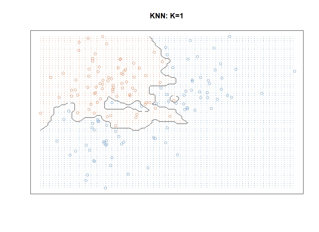
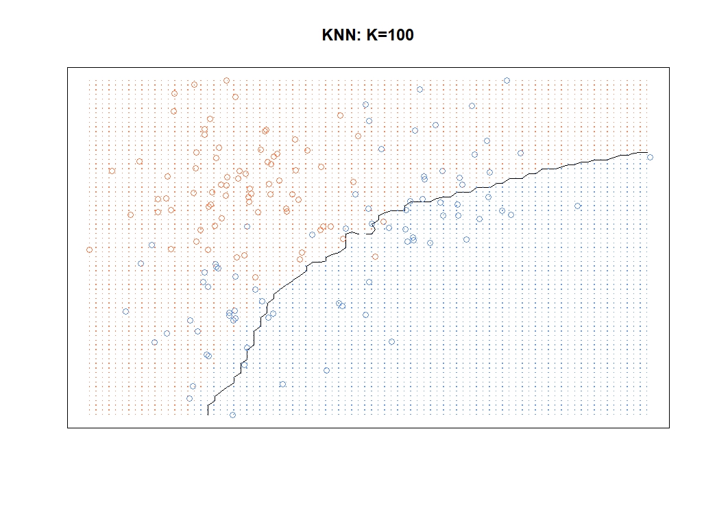
We will typically start by choosing \(k=\sqrt{\text{\# of Observations}}\), but different values of \(k\) will result in different predictions. Additionally, small values of \(k\) might lead to overfitting the training set (low bias and high variance) while high values of \(k\) might lead to a very “rigid” model (high bias and low variance). An example of this can be seen below:
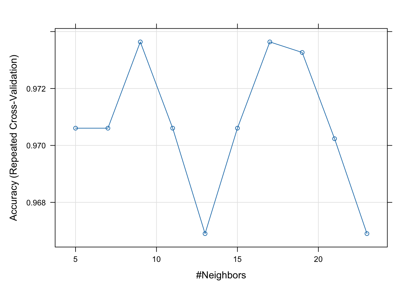
We can determine which \(k\) value is best by running cross-validation on each \(k\) value. We can look for when the accuracy stops climbing, which is around 9 in our case. It has not been an issue so far, but when we run the KNN, we will want to make sure to scale and center the data, which can be done using the scale() function. This is because if we are dealing with variables with different units the distances may over-emphasize certain predictors.
k-Nearest Neighbors

100 samples
  2 predictor
  3 classes: 'setosa', 'versicolor', 'virginica'

Pre-processing: centered (2), scaled (2)
Resampling: Cross-Validated (10 fold, repeated 3 times)
Summary of sample sizes: 90, 91, 90, 90, 90, 91, ...
Resampling results across tuning parameters:

  k   Accuracy   Kappa
   5  0.9706061  0.9556683
   7  0.9706061  0.9556683
   9  0.9736364  0.9601951
  11  0.9706061  0.9556683
  13  0.9669024  0.9501128
  15  0.9706061  0.9556683
  17  0.9736364  0.9601174
  19  0.9732660  0.9596123
  21  0.9702357  0.9550856
  23  0.9669024  0.9500351

Accuracy was used to select the optimal model using the largest value.
The final value used for the model was k = 17.