As you go about your day, you make decisions, without really even thinking about it, based on if certain criteria are met. For instance, as a studious data scientist, you may come across the dilemma of deciding whether or not to go to a party on Friday night. If you have homework then you will stay home (…right guys?!?) and if you have no homework then you will only go if a friend is going. This sort of decision-making process (using “yes/no” questions or “what-if” scenarios) is the idea of decision trees. Decision Trees are a machine learning model that is easy to interpret because it makes decisions in the same way humans make decisions.
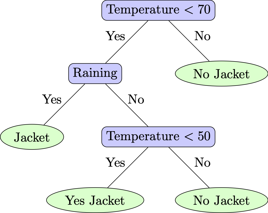
Below is an example of a decision tree that someone might use to determine if they should wear a jacket when they leave the house. The first question they ask themselves is whether the temperature is below 70 degrees or not. If it is not less than 70 degrees then they will not wear a jacket, but if it is less than 70 degrees then they determine if it will be raining during the day. If it is raining then they wear a jacket, if it is not then they will wear a jacket if it is less than 50 degrees and go without a jacket if it is not less than 50 degrees:
When reading about decision trees you may come across terminology such as “root node”, “decision nodes”, “leaf nodes” and “branches”. The “root node” is where you start the decision-making process while the “decision nodes” are the choices you make and the “leaf node” is the classification you end up with. The “branches” are the competing outcomes.
11.2 Choosing Splits
The splits in the tree are determined by which split creates the best division and results in the lowest entropy (which is a measure of purity). A split with high entropy results in very diverse groups and little gained information but a split with low entropy helps divide our data into different categories and results in a high information gain split. The formula for entropy is the following where \(c\) is the number of classifications at the split and \(p_i\) is the proportion of values falling into class level \(i\): \[\text{Entropy} = \sum_{i=1}^c -p_i\cdot \log_2(p_i)\]
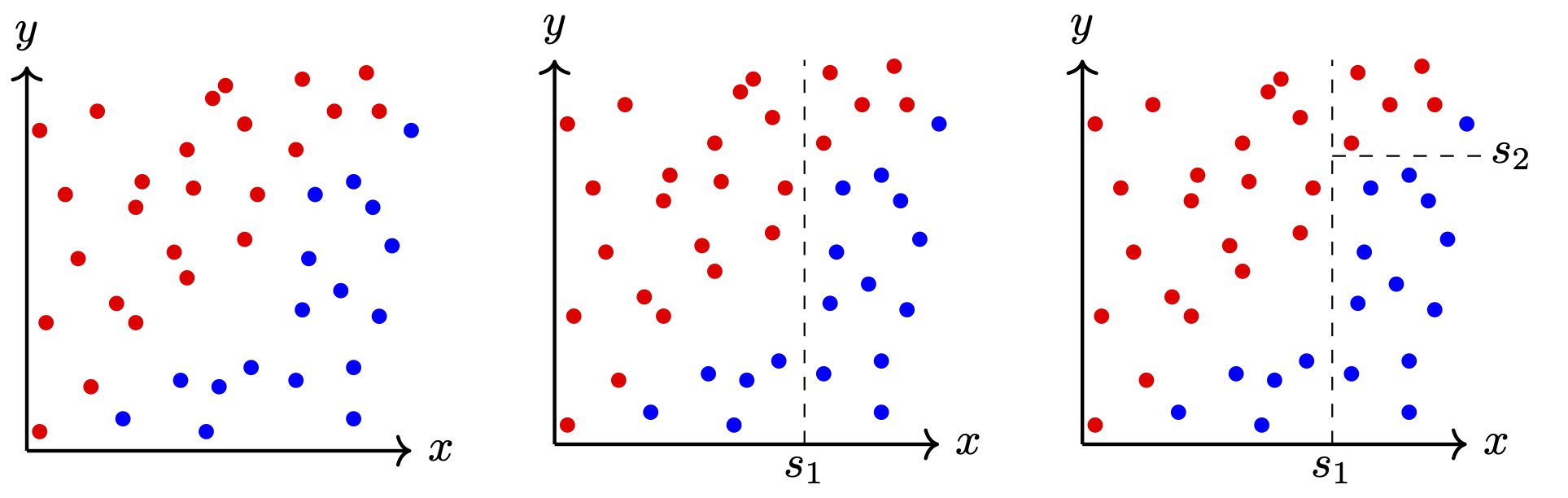
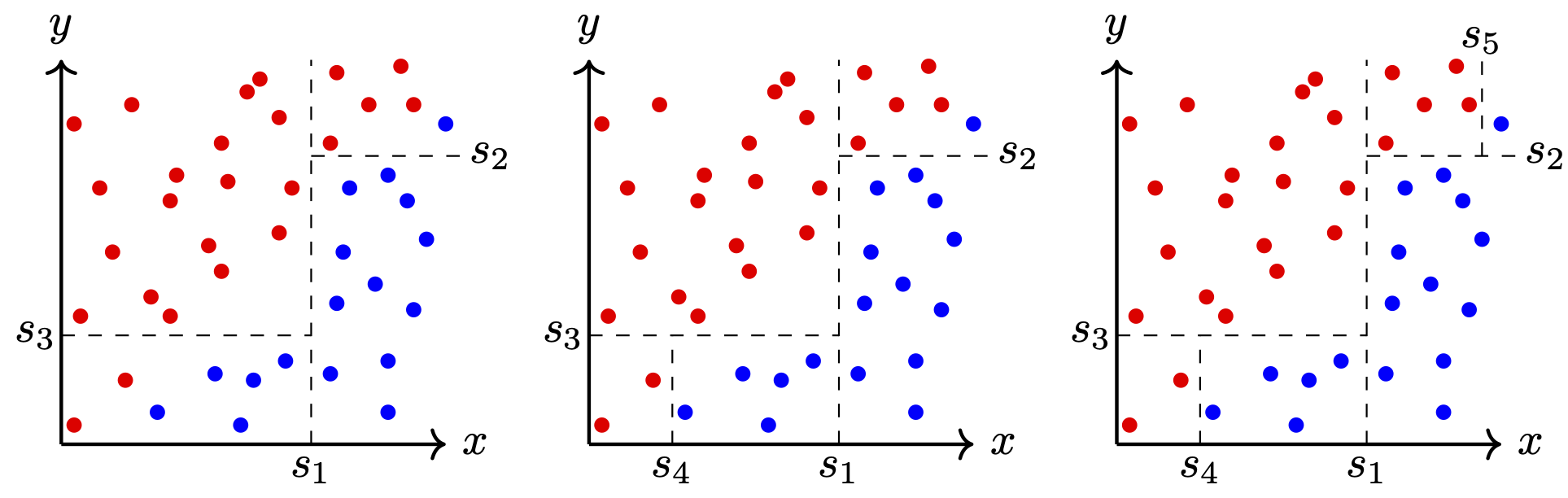
Notice that the entropy will be equal to 0 when the splits result in homogeneous groups and 1 when they result in perfectly even groupings.An example of how the splits are performed can be seen below. Notice how each split tries to make each group as “pure” as possible:
We can use entropy to determine where the splits (\(s_i\)) would go in the graph. We will have the computer do these since there are a great deal of possible options, so we show this math just as an example. Starting out, the overall set has 17 Blue and 25 Red resulting in an entropy of: \[\text{Entropy}_\text{Parent} = - \frac{17}{42} \cdot \log_2\left( \frac{17}{42}\right) - \frac{25}{42} \cdot \log_2\left( \frac{25}{42}\right) = 0.974\]
With the split \(s_1\) we break the data into 2 groups, one of which has 25 observations (20 Red and 5 Blue) and another has 17 observations (12 Blue and 5 Red). We can then calculate the entropy of each group and weigh them according to how many observations are in each. We then use this weighted entropy to calculate the information gained. We will try different splits and take the one with the most information gained:
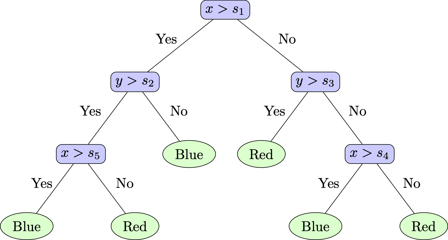
After we have created these splits and are left with “pure” groupings, we can construct a decision tree to model this information. Note that it is customary to have the left branch represent “yes” and the right branch represent “no”.
11.3 Building a Decision Tree in R
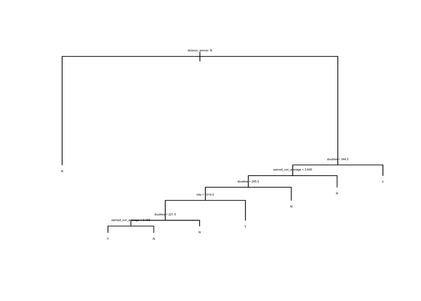
In order to do this in R, we can use the tree() function in the tree library. We will build the model in a similar way to how we have built models previously. As we can see from this model, the misclassification rate is only 3.6%. We can also visualize the decision tree by plotting the model and then adding the text to the tree (though it is not the most visually appealing tree):
When we make decision trees, it is very easy to underfit and overfit our data. How well our model fits the data will rely on how deep our tree is (that is the number of layers we have for the tree). Having a tree with only a few splits would underfit the data and lead to high bias and low variance while having a tree with hundreds of splits would overfit the data and lead to low bias and high variance. Luckily though, we can “prune” the tree to determine a possible best length. The code below builds a full model and then we will show how to prune it. We will be looking at the “mlb_teams” dataset in the openintro library. First, we need to do a little house-keeping in order to work with the data and build our model:
Classification tree:
tree(formula = world_series_winner ~ ., data = mlb_train)
Variables actually used in tree construction:
[1] "division_winner"    "wins"               "doubles"
[4] "homeruns"           "earned_run_average" "hits"
[7] "errors"
Number of terminal nodes:  18
Residual mean deviance:  0.09738 = 101.2 / 1039
Misclassification error rate: 0.02176 = 23 / 1057
pred <-predict(mlb_tree, mlb_test, type ="class")table(mlb_test$world_series_winner, pred)
   pred
      N   Y
  N 334   8
  Y   9   2
As we can see above, there are entirely too many nodes (24 nodes!!!) and layers for it to be easily interpretable. We are getting into the area of overfitting our data with all of the conditions that we used (the training error is 2% and the testing error is 7%). We can “prune” the tree to avoid overfitting.
11.5 Pruning Decision Trees
This is done with cross-validation to determine which would be best. We will look for the size associated with the smallest dev value (which is the number of cross-validation errors). For our example we will not use the recommendation since it is a single node, we will use the next “best” one which is 8 nodes. This is caused for us in this example because so few observations are in the positive class (“winning the world series”) that it is easiest just to say everyone lost.
mlb_cv_tree <-cv.tree(mlb_tree, FUN = prune.misclass)mlb_cv_tree