15  Neural Networks

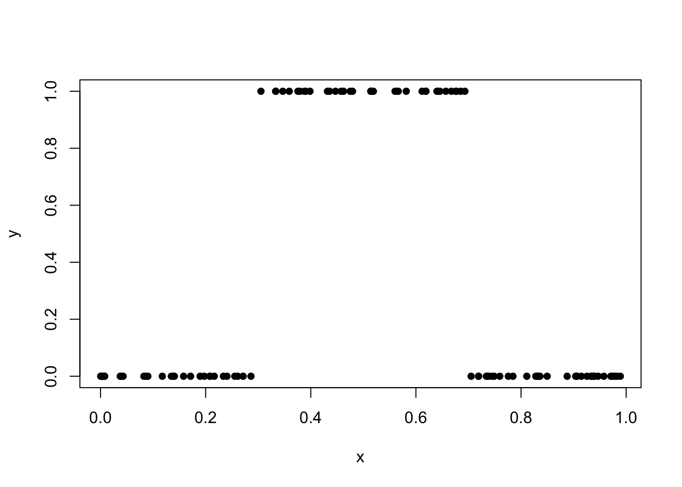
Neural networks are a machine learning model that is often described as a “black box”, meaning it is sometimes hard to explain and interpret what it is doing behind the scenes. The basic idea of the model was inspired by the structure of the brain as it has a multitude of interconnected “neurons” (often a non-linear mathematical function that takes an input and produces an output). Each connection has different weights and biases which are adjusted as the model is trained.

15.1 Neural Network Structure

Before diving into the specifics of the model, we should first go over some terminology. In the diagram seen below each circle is a neuron (or node) that takes an input, processes it using a non-linear function, and then passes the output to the next neuron. The input layer is where we pass in the data, and the hidden layers are where the computations happen. The output layer produces the final result. There can be multiple hidden layers within the model along with as many or few nodes within each layer. Each connection between neurons has a weight that controls the influences of the neuron’s output on the next neuron along with a bias that helps the model to better fit the data.

15.2 Activation Functions and Forward Propagation

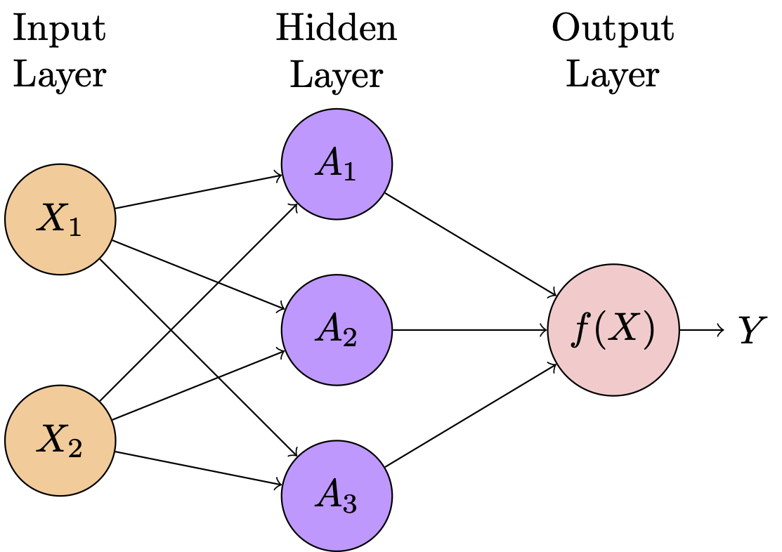
Using the diagram above as an example, we have \(X_1\) and \(X_2\) as our input data. These values will be passed to the first hidden layer, with each value being passed into each node of the layer. Each neuron in the hidden layer will then perform a series of operations on the inputs of the previous layer. This is done through the process of a weighted sum, with the inputs being multiplied by some weight and a bias added to it: \[z= (w_1 \cdot x_1) + (w_2 \cdot x_2) + b\]

This weighted sum (\(z\)) is then passed through an activation function which represents a transformed version of the input layer. Typical activation functions include the sigmoid function (\(\frac{1}{1 + e^{-z}}\)), Tanh function, and softmax function, along with a few others. This transformed value then acts as the input for the next layer. This process is repeated for each node/layer until the output layer which then once again takes the inputs, passes it through the activation function, and produces an output. The sigmoid function will be good for binary classification while the softmax function will be good for multi-level classifications. Additional activation functions can be used for regression.

15.3 Building Neural Networks in R

Let’s look at an example in R to get a better understanding of how this works. We will use the neuralnet() function within the neuralnet library. To generate our data we will randomly sample 100 values (\(x\)) between 0 and 1 and then determine the output value (\(y\)) based on where it is. Notice that we could not do linear regression or logistic regression on this data based on its non-linear nature.

library(neuralnet)
set.seed(42) # Answer to Life, the Universe, and Everything
data <- data.frame(x = runif(100, 0, 1))
data$y <- ifelse(data$x > 0.3 & data$x < 0.7, 1, 0)
plot(data, pch=16)

# hidden=c(2) indicates 1 layer with 2 nodes
model <- neuralnet(y ~ x, data = data, hidden = c(2), 
                     act.fct = "logistic", linear.output = FALSE)
plot(model)

The code and output above show us the neural network pertaining to our data. Note that if we wanted multiple layers with multiple nodes we could specify that in the hidden argument. For instance, if we wanted 3 layers with 3, 5, and 2 nodes in it respectively we would specify hidden=c(3,5,2). Looking at the model plot above, we could determine what a value would be classified as. Let’s run through this example using \(x=0.9\) and the weights from the picture above. Note that the output value is roughly the same (the slight difference is due to rounding error) and that instead of using the predict() function we will instead use the compute() function. This will give us a variety of information, with $net.results giving us the output value. Using this predicted probability you could then create a threshold to classify values as 0 or 1:

x <- 0.9 # Starting Value

z1 <- -13.93391*x + 3.88369
a1 <- 1/(1+exp(-z1))
a1 # Value of first neuron

[1] 0.0001739047

z2 <- -9.20548*x + 5.95377
a2 <- 1/(1+exp(-z2))
a2 # Value of second neuron

[1] 0.08857481

z3 <- -96.0148*a1 + 72.47466*a2 - 27.34587
a3 <- 1/(1+exp(-z3))
a3 # The output value

[1] 8.026213e-10

compute(model, data.frame(x=0.9))

$neurons
$neurons[[1]]
         x
[1,] 1 0.9

$neurons[[2]]
     [,1]         [,2]       [,3]
[1,]    1 0.0001739037 0.08857497


$net.result
             [,1]
[1,] 8.026319e-10

We could then compute the predicted probability for a sequence of \(x\) values in order to plot a line showing the results:

test_data <- data.frame(x = seq(0, 1, length.out = 100))
predictions <- compute(model, test_data)
test_data$predicted_y <- predictions$net.result
 
plot(data$x, data$y, col = "blue", pch = 16, 
     main = "Neural Network with Sigmoid Activation Function",
     xlab = "x", ylab = "y (0 or 1)")
lines(test_data$x, test_data$predicted_y, col = "red", lwd = 2)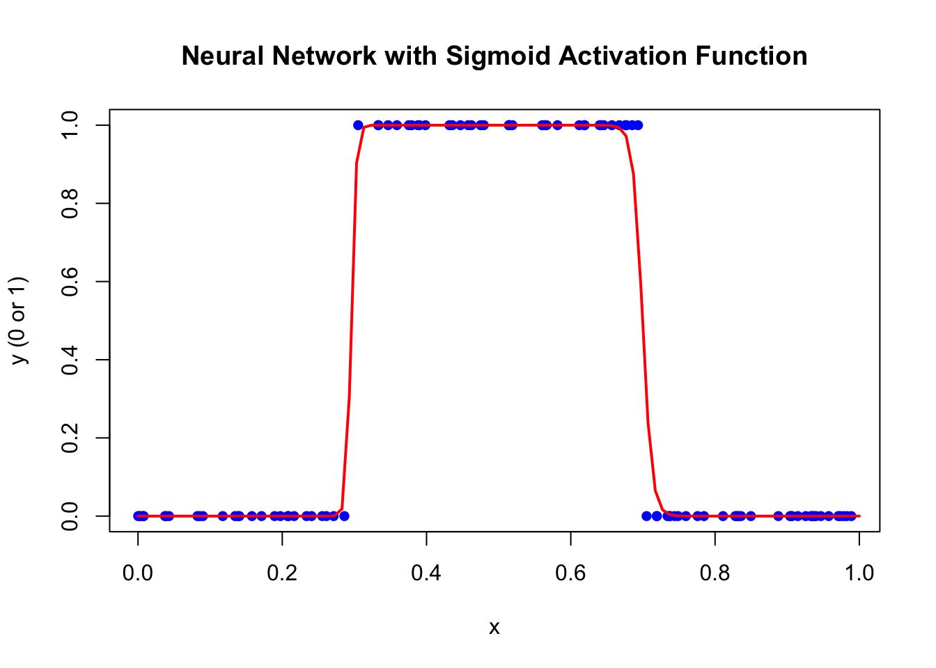

15.4 Neural Networks for Regression

This could also be done to model non-linear data which may require a more complex model:

set.seed(42) # Answer to Life, the Universe, and Everything
data <- data.frame(x = runif(100, 0, 1))
data$y <- sin(2 * pi * data$x) + rnorm(100, sd = 0.1)
plot(data, pch=16)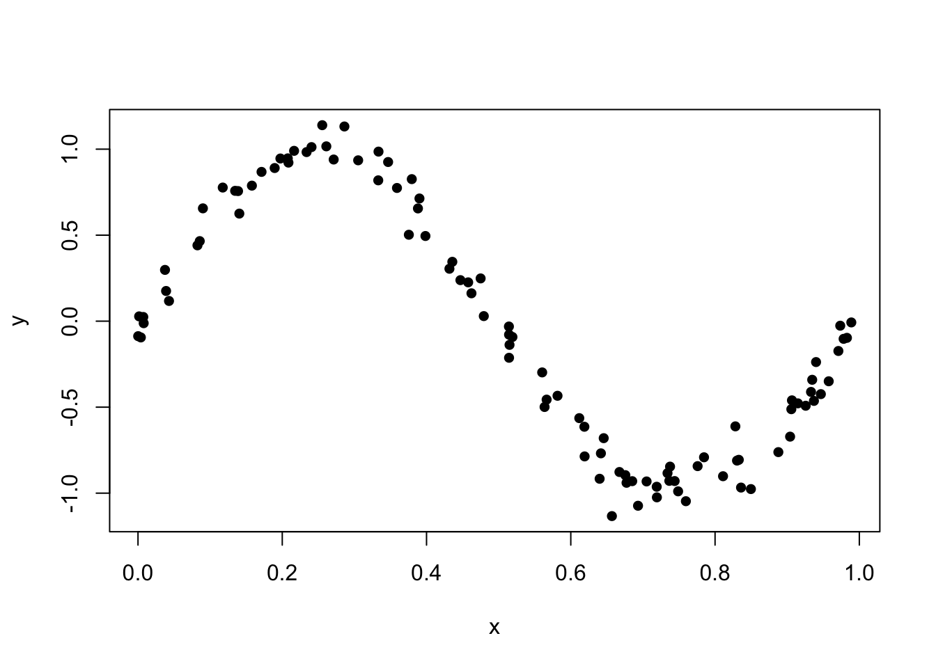

model <- neuralnet(y ~ x, data = data, hidden = c(5, 3), 
                   linear.output = TRUE)
plot(model)

test_data <- data.frame(x = seq(0, 1, length.out = 100))
predictions <- compute(model, test_data)
test_data$predicted_y <- predictions$net.result
 
plot(data$x, data$y, col = "blue", pch = 16, 
     main = "Neural Network Regression with Linear Activation",
     xlab = "x", ylab = "y (Continuous Output)")
lines(test_data$x, test_data$predicted_y, col = "red", lwd = 2)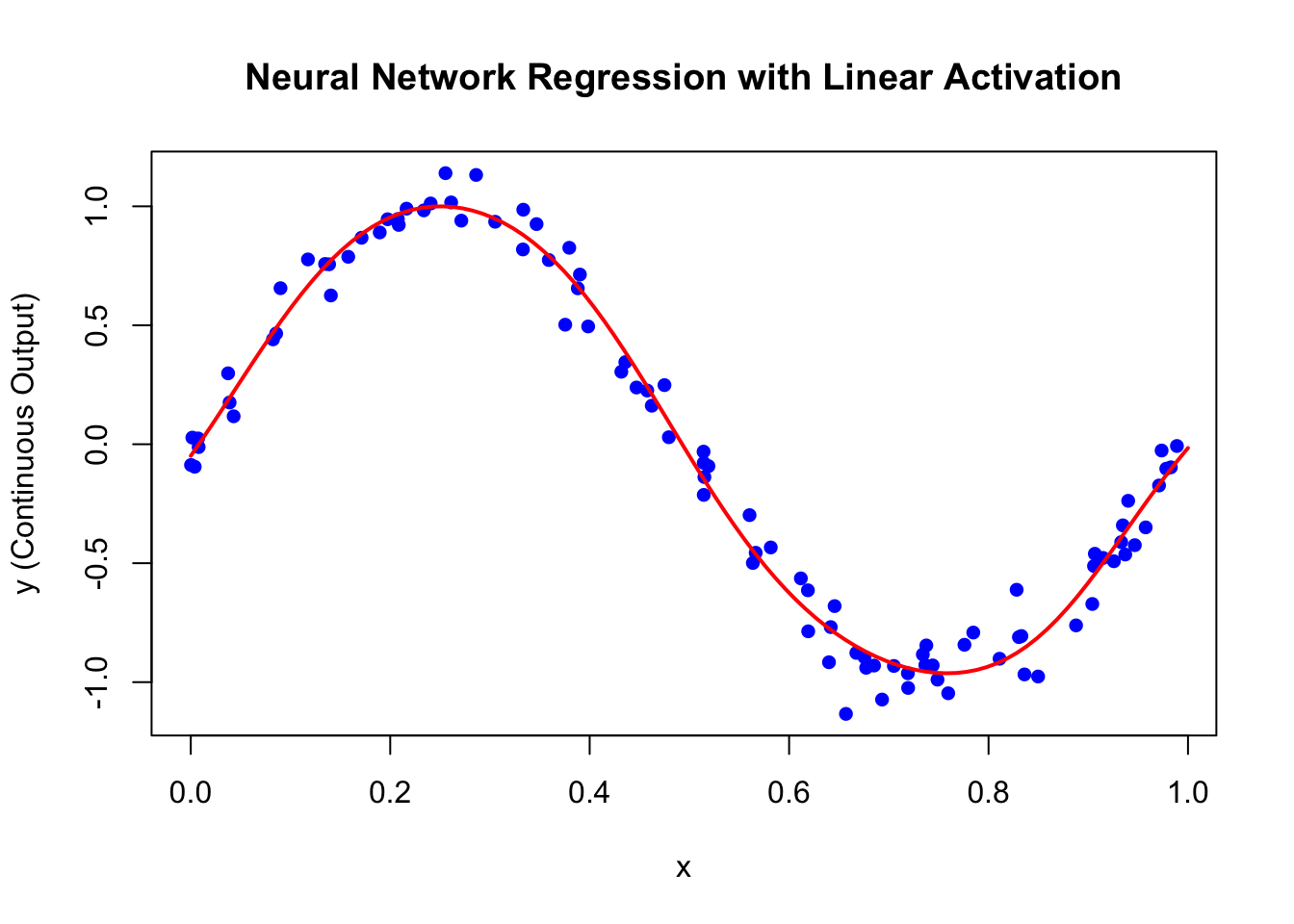

One last final example we will see is a more abstract regression problem. If we would like to predict the weight of a baby in the babies dataset we could do it as follows (with a linear example as a baseline. The data is scaled and 2 layers are used to run the model. WARNING: The package we are using is not the optimal package and can be very computationally intensive. We are using this package because it is easy to use for beginners. Choosing multiple layers/nodes may result in the model taking a long time to run. As a word of caution, choose basic models and then slowly increase the size to make sure it will not take too long to run:

set.seed(123)
library(openintro)
data("babies")
babies1 <- na.omit(babies)
babies1 <- scale(babies1)

train_index <- sample(1:nrow(babies1), 0.75*nrow(babies1),replace=FALSE)
train <- data.frame(babies1[train_index,])
test <- data.frame(babies1[-train_index,])

linear_model <- lm(bwt ~ gestation + height + weight, data=train)
pred_linear <- predict(linear_model, newdata=test)
rmse_linear <- sqrt(mean((pred_linear - test$bwt)^2))
rmse_linear

[1] 0.913985

nn_model <- neuralnet(bwt ~ gestation + weight + height, data=train, 
                      hidden=c(3,2), linear.output=TRUE, stepmax=1e07)

pred_nn <- compute(nn_model, test)$net.result
rmse_nn <- sqrt(mean((pred_nn - test$bwt)^2))
rmse_nn

[1] 0.9160642