So far, we have discussed how to implement, interpret, and make predictions using a Simple Linear Regression model. In this lecture, we will take a deeper look into validating our assumptions so that it makes sense to use a linear model on our data as well as make inferences from our coefficients. The assumptions that we will discuss include the linearity of our data, normality of the residuals, and constant variance. We will also investigate values that are outliers or have high leverage/influence on the model. And finally, we will end the write-up by discussing prediction and confidence intervals pertaining to the model.
2.1 Data is Linear in Nature
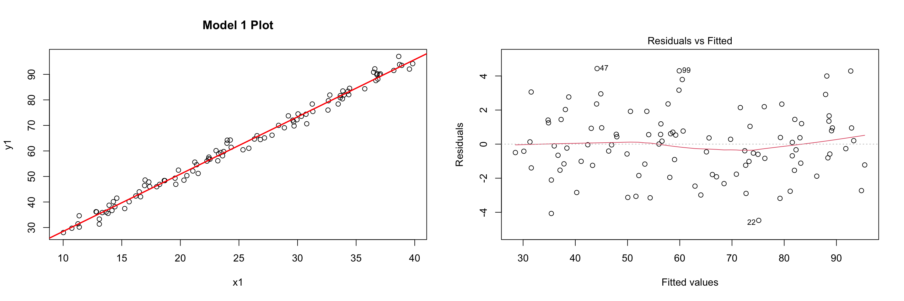
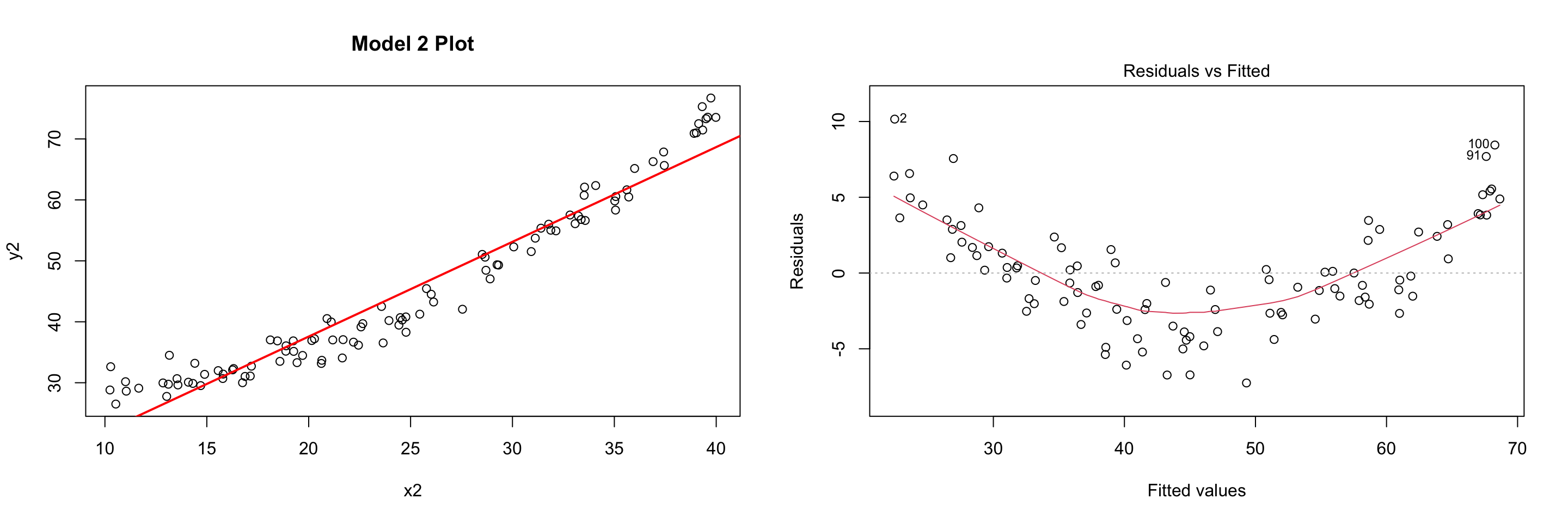
The first assumption that we should always check is that our data follows a linear pattern. Just looking at the summary outputs will not tell us the whole story. For instance, the two models below both appear to be highly significant and both models have very high \(R^2\) values, indicating both models would do a good job making predictions. But, as we will see, one of them is linear and one is not. Note that the output has been edited for space reasons:
summary(mod1)
Call:
lm(formula = y1 ~ x1)

Residuals:
    Min      1Q  Median      3Q     Max
-4.4759 -1.2265 -0.0395  1.1927  4.4345

Coefficients:
            Estimate Std. Error t value Pr(>|t|)
(Intercept)  6.04197    0.60085   10.06   <2e-16 ***
x1           2.24401    0.02279   98.47   <2e-16 ***
---
Signif. codes:  0 '***' 0.001 '**' 0.01 '*' 0.05 '.' 0.1 ' ' 1

Residual standard error: 1.939 on 98 degrees of freedom
Multiple R-squared:   0.99, Adjusted R-squared:  0.9899
F-statistic:  9697 on 1 and 98 DF,  p-value: < 2.2e-16
summary(mod2)
Call:
lm(formula = y2 ~ x2)

Residuals:
    Min      1Q  Median      3Q     Max
-7.2537 -2.4408 -0.4522  2.3879 10.1574

Coefficients:
            Estimate Std. Error t value Pr(>|t|)
(Intercept)  6.48355    1.07774   6.016 3.09e-08 ***
x2           1.55480    0.04102  37.903  < 2e-16 ***
---
Signif. codes:  0 '***' 0.001 '**' 0.01 '*' 0.05 '.' 0.1 ' ' 1

Residual standard error: 3.598 on 98 degrees of freedom
Multiple R-squared:  0.9361,    Adjusted R-squared:  0.9355
F-statistic:  1437 on 1 and 98 DF,  p-value: < 2.2e-16
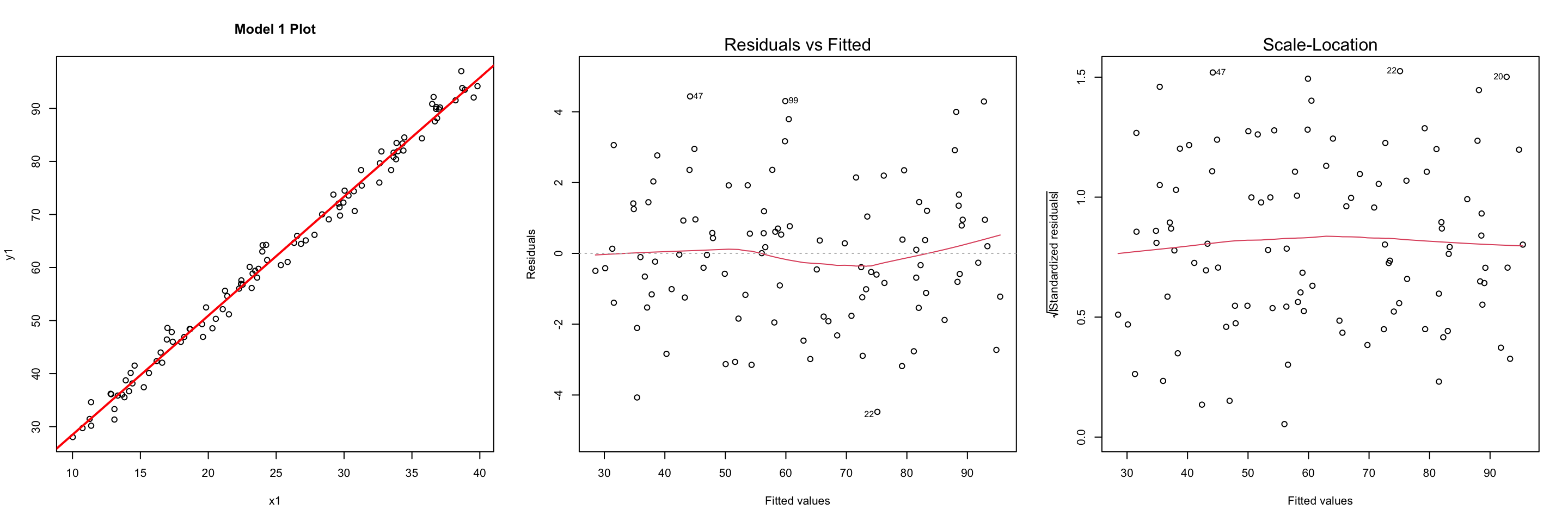
To validate the linearity of our model we will not only want to look at the plotted data, but also the residual plot. This is a plot that compares the fitted values to the residual values. This can be done by passing the model into the plot() function and using the which=1 argument. What we are looking for in this visualization is a plot with no identifiable pattern. If a pattern exists then it may indicate our data is not linear.
As we can see in the plots above, the first model appears to be linear in nature. The residual plot shows no discernible pattern, leading us to believe that the data is linear since points fall above and below the line of best fit “randomly”. On the other hand, it appears that the second model is not linear. If we look at the residual plot we can see a clear pattern, meaning the model has violated our assumption of linearity. If we notice on the original plot, when \(x\) is small all of the points are above the line of best fit, in the middle they all fall below the line of best fit, and when \(x\) is large they are again above the line of best fit, leading to the residual plot to be quadratic in nature.
2.2 Residuals are Normally Distributed
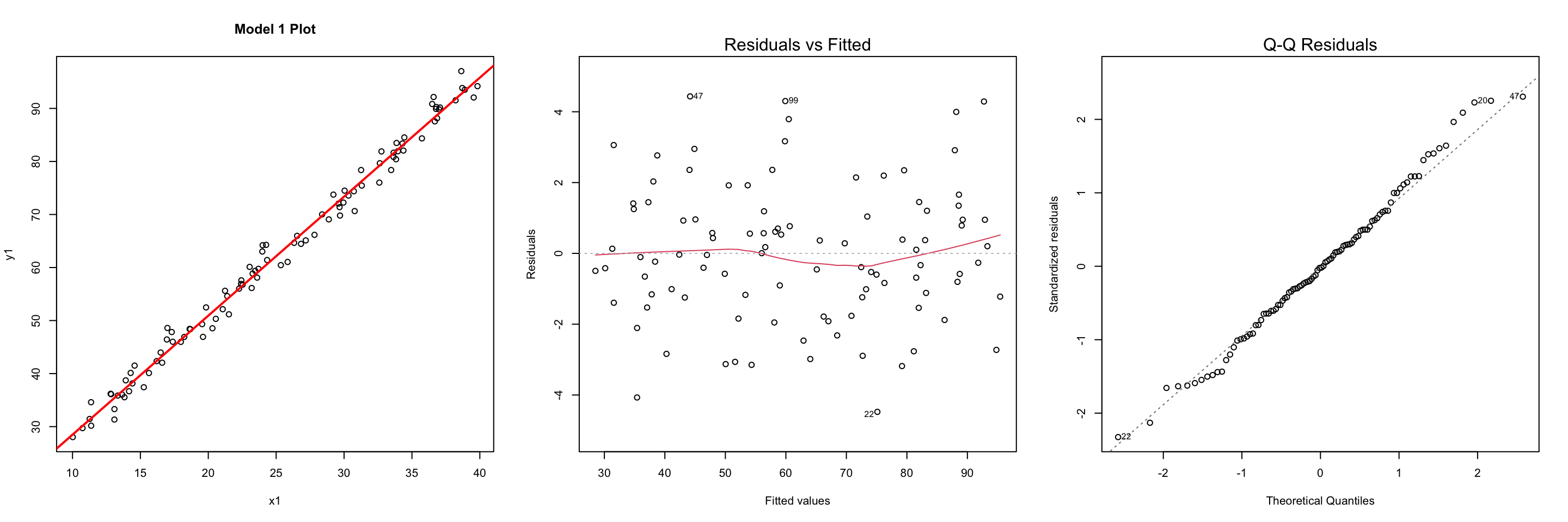
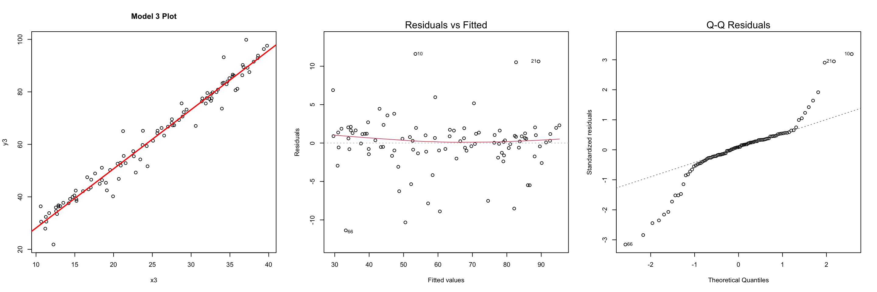
The second assumption we will want to validate is that residuals are normally distributed. To do this, we will look at a “QQ Plot” of the residuals. As a reminder, the QQ Plot compares the quantiles of the data and the quantiles of a normal distribution. If the data follows a normal distribution then the plot should roughly be a straight line. If there is a significant deviation from the line (especially in the tails) then we would question the normality of the data. The plot() function will do it for us if we specify the argument which=2 when we pass in the model.
In the two models shown below, we can see that both are linear in nature and both are highly significant with great \(R^2\) values. But, when we look at the QQ Plot we can see that Model 3 violates the normal assumption for residuals. Without the normality assumption, we will have a difficult time making confidence intervals and performing hypothesis testing.
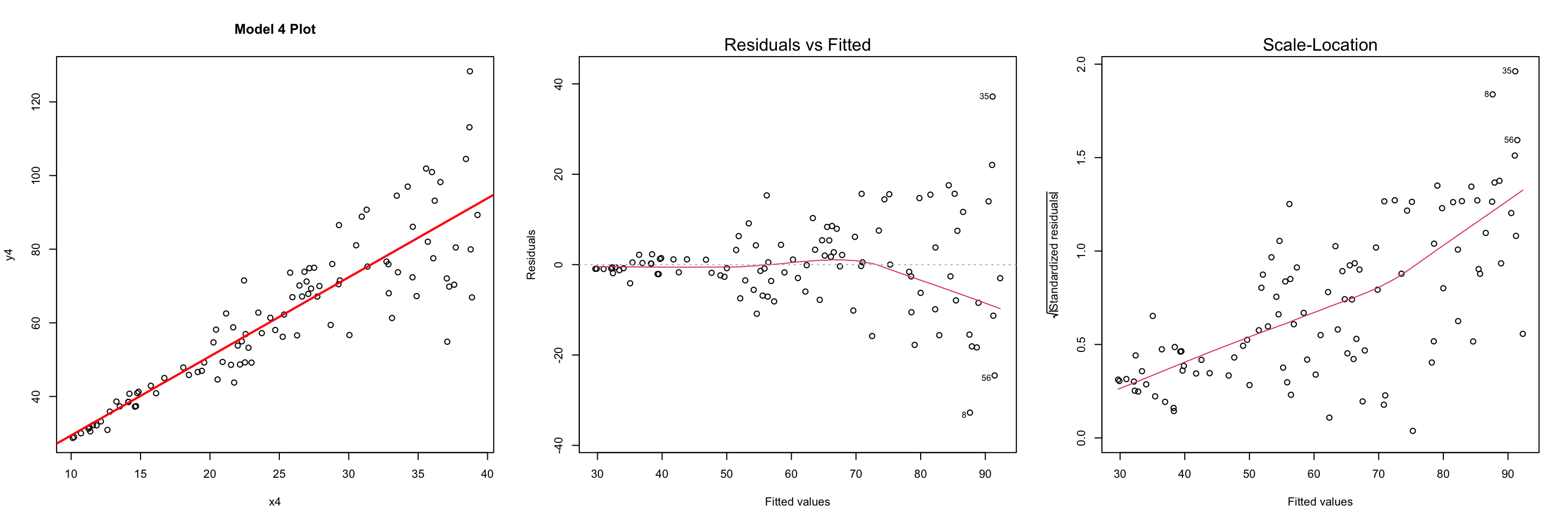
The third assumption we will want to verify is that we have a constant variance. To do this, we will look at our plot, our residual plot, and the scale-location plot. Ideally, the scale-location plot will have a horizontal line and randomly spread out points. In the two models below, we can see that Model 1 appears to be randomly spread out but when we look at Model 4 we can see a non-horizontal line. And then looking at the original plot and residuals we can see the variance “fans” out, showing us we do not meet the assumption of constant variance. This indicates that Model 4 exhibits heteroskedasticity (non-constant variance).
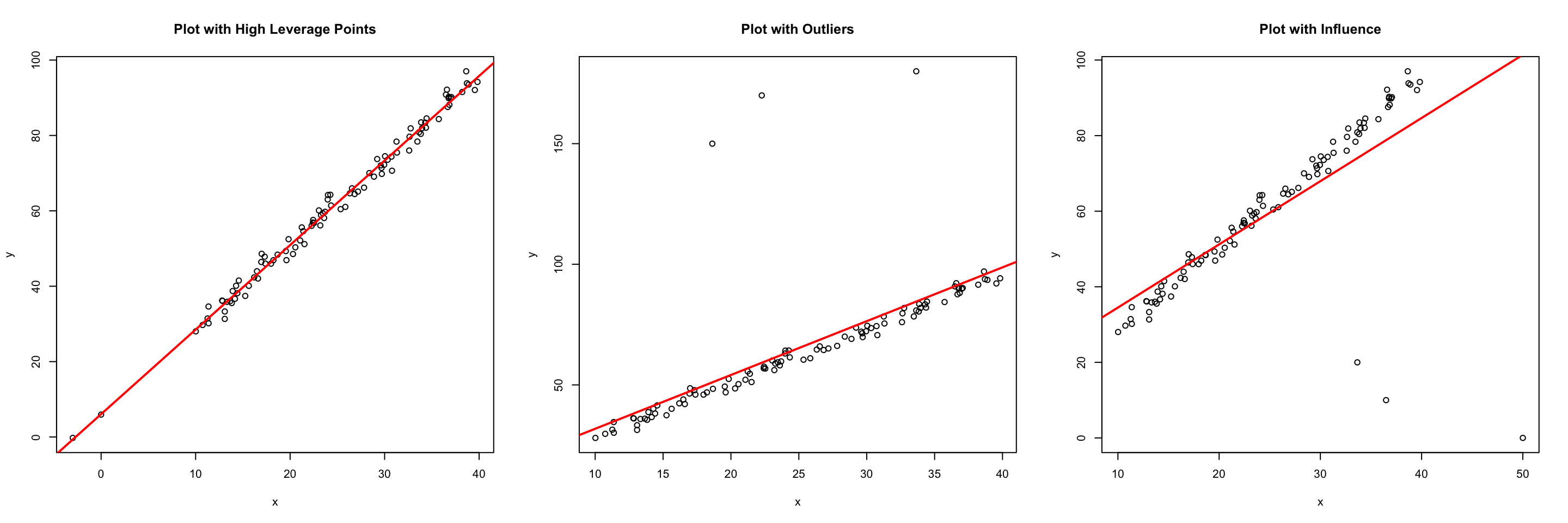
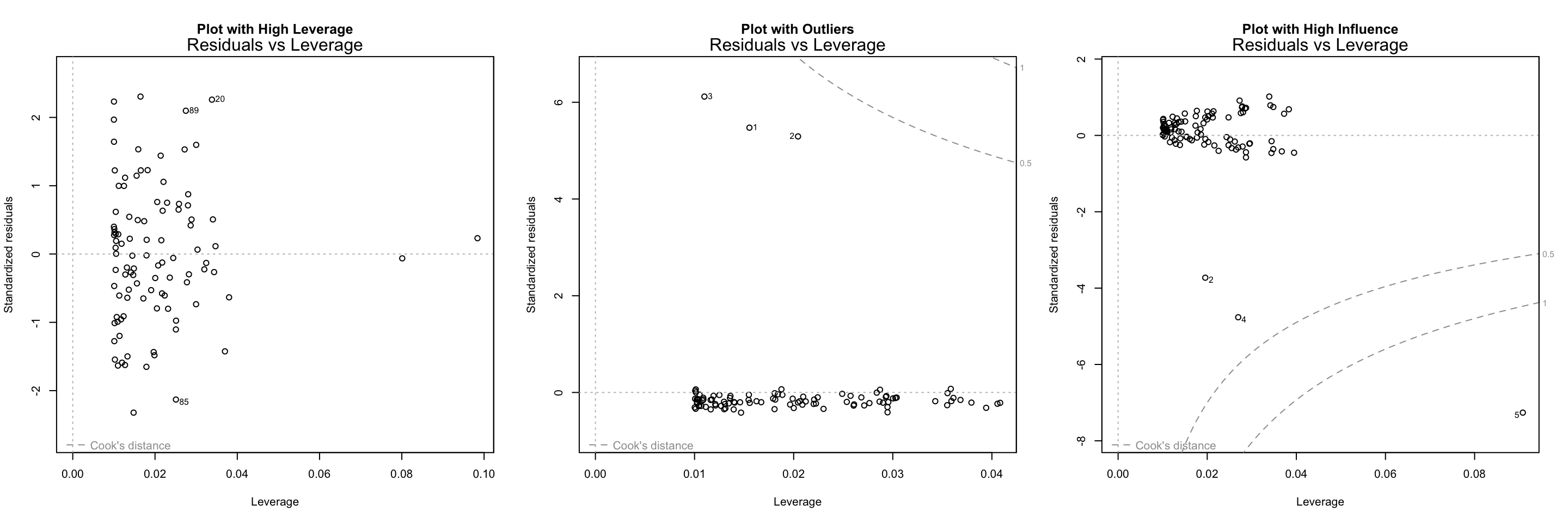
Next, we will want to discuss the effects of outliers on our dataset. An outlier is any value that is not predicted well by the fitted regression model. We will see that some outliers have a large effect on our linear model and some have no effect at all. To better understand this idea, we will introduce leverage and influence. Values with high leverage are ones that fall far outside of the range of the other feature values. Values with high influence have a disproportionate impact on our regression results. The visualization below should help exhibit what each case may look like. Points can have a combination of all 3 characteristics.
If we look at a summary of the model for the original data, the model with the added high leverage point, the model with the outliers, and the model with the high influence point, we can see how each may affect the coefficients and \(R^2\) values. Notice that the model with the high leverage point is virtually identical to the original model. This is because the added high leverage point is not influential since it lies on the line of best fit. The model with the outliers added are not high leverage, but they are somewhat influential as we can see the intercept coefficient change along with a drop in the \(R^2\) value. Finally, notice that the model with high influence (which also happens to have a high leverage point) alters the model substantially than when there is a low-influence high leverage point. Both the coefficients are drastically different along with a substantial drop in the \(R^2\) value.
summary(original_model)
Call:
lm(formula = y ~ x)

Residuals:
    Min      1Q  Median      3Q     Max
-4.4759 -1.2265 -0.0395  1.1927  4.4345

Coefficients:
            Estimate Std. Error t value Pr(>|t|)
(Intercept)  6.04197    0.60085   10.06   <2e-16 ***
x            2.24401    0.02279   98.47   <2e-16 ***
---
Signif. codes:  0 '***' 0.001 '**' 0.01 '*' 0.05 '.' 0.1 ' ' 1

Residual standard error: 1.939 on 98 degrees of freedom
Multiple R-squared:   0.99, Adjusted R-squared:  0.9899
F-statistic:  9697 on 1 and 98 DF,  p-value: < 2.2e-16
summary(leverage_model)
Call:
lm(formula = y ~ x)

Residuals:
    Min      1Q  Median      3Q     Max
-4.4670 -1.2119 -0.0786  1.1969  4.4313

Coefficients:
            Estimate Std. Error t value Pr(>|t|)
(Intercept)  6.06004    0.54857   11.05   <2e-16 ***
x            2.24314    0.02103  106.67   <2e-16 ***
---
Signif. codes:  0 '***' 0.001 '**' 0.01 '*' 0.05 '.' 0.1 ' ' 1

Residual standard error: 1.938 on 98 degrees of freedom
Multiple R-squared:  0.9915,    Adjusted R-squared:  0.9914
F-statistic: 1.138e+04 on 1 and 98 DF,  p-value: < 2.2e-16
summary(outlier_model)
Call:
lm(formula = y ~ x)

Residuals:
    Min      1Q  Median      3Q     Max
 -7.539  -4.380  -3.251  -1.832 110.811

Coefficients:
            Estimate Std. Error t value Pr(>|t|)
(Intercept)   9.5066     5.6445   1.684   0.0953 .
x             2.2310     0.2141  10.421   <2e-16 ***
---
Signif. codes:  0 '***' 0.001 '**' 0.01 '*' 0.05 '.' 0.1 ' ' 1

Residual standard error: 18.21 on 98 degrees of freedom
Multiple R-squared:  0.5257,    Adjusted R-squared:  0.5208
F-statistic: 108.6 on 1 and 98 DF,  p-value: < 2.2e-16
summary(influence_model)
Call:
lm(formula = y ~ x)

Residuals:
     Min       1Q   Median       3Q      Max
-101.386   -1.937    1.876    6.128   14.648

Coefficients:
            Estimate Std. Error t value Pr(>|t|)
(Intercept)   17.775      4.436   4.007  0.00012 ***
x              1.672      0.167  10.013  < 2e-16 ***
---
Signif. codes:  0 '***' 0.001 '**' 0.01 '*' 0.05 '.' 0.1 ' ' 1

Residual standard error: 14.64 on 98 degrees of freedom
Multiple R-squared:  0.5057,    Adjusted R-squared:  0.5007
F-statistic: 100.3 on 1 and 98 DF,  p-value: < 2.2e-16
If you wanted to learn more about how we would determine if a point has high leverage we would need to do some linear algebra. To become an expert in machine learning, one should learn linear algebra and statistics. But, we will not concern ourselves with the theory of this derivation, but I will include it for the curious student: Assuming we wrote the linear model as \(\mathbf{Y}=\mathbf{X}\beta + \epsilon\), where \(\mathbf{X}\) and \(\mathbf{Y}\) are matrices, then we could derive the coefficients as \(\hat{\beta}=(\mathbf{X}^T\mathbf{X})^{-1}\mathbf{X}^T\mathbf{Y}\) and the predicted values as \(\hat{\mathbf{Y}} = \mathbf{X}(\mathbf{X}^T\mathbf{X})^{-1}\mathbf{X}^T\mathbf{Y}\). We can then calculate the leverage matrix \(\mathbf{H}\) (called the Hat matrix) as \(\mathbf{H}=\mathbf{X}(\mathbf{X}^T\mathbf{X})^{-1}\mathbf{X}^T\). This allows us to see how much weight each observation adds to the model with \(\hat{y_i}=h_1y_1 + h_2y_2 + \cdots + h_ny_n\). We will say that points are high leverage values if \(h_i > 2\sqrt{\frac{p+1}{n-p-1}}\) where \(n\) is the number of observations and \(p\) is the number of coefficients.
We can determine if a point is highly influential by calculating the Cook’s Distance. This helps us summarize how much the regression model changes when the \(i^\text{th}\) observation is removed. This can be calculated as \(D_i = \frac{\sum(\hat{y_j} - \hat{y}_{j(i)})^2}{p\times \text{MSE}}\). We then flag an observation as influential if \(D_i > \frac{4}{n}\). This can be done in R using the cooks.distance() function.
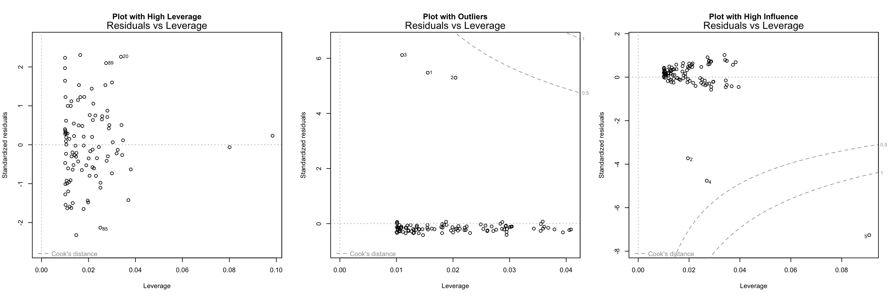
Luckily, we do not have to do any of these calculations, we will just need to look at the Residual vs Leverage Plot to make a determination of which observations exhibit high leverage and/or high influence. Any observation that has a standardized residual less than -2 or greater than 2 might be considered an outlier. The \(x\)-axis shows which values have high leverage (values on the right side), and values on the top or bottom right would be considered influential. R will also label 3 of the observation numbers which are the most influential. This visualization will require us to use which=5 when we plot the model.
par(mfrow=c(1,3))plot(leverage_model, which=5, main="Plot with High Leverage")plot(outlier_model, which=5, main="Plot with Outliers")plot(influence_model, which=5, main="Plot with High Influence")
2.5 Confidence vs. Prediction Intervals
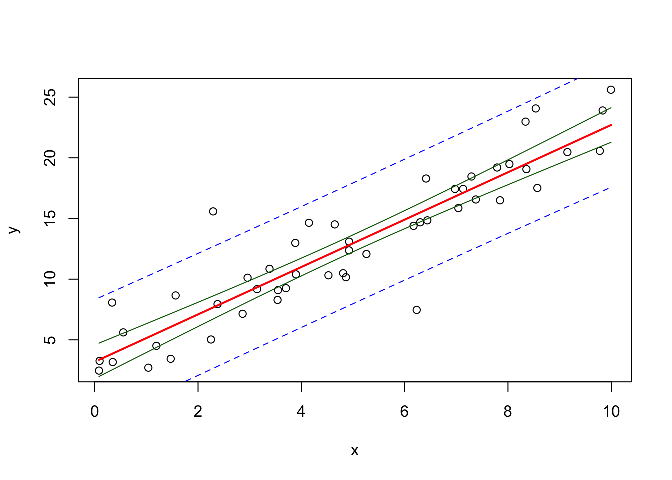
Finally, the last things we will discuss are confidence intervals and prediction intervals. The 95% Confidence Interval will tell us the interval in which we are 95% confident where the true line of best fit is. On the other hand, the 95% Prediction Interval will tell us the interval in which 95% of the values will be. We can think of it as the prediction interval allows us to predict where a value may fall, while the confidence interval tells us where the mean value at a given point may be. So, the prediction interval will always be wider than the confidence interval. We can calculate both of these using the predict() function in R. We can specify what type of interval we wish to obtain (confidence/prediction) along with the level we want (95% = .95). To do so, we still need to pass it new \(x\) values, which I created using the seq() function. I encourage you to run this line by line yourself and at each stage display the variable to get an idea of what the function is doing.