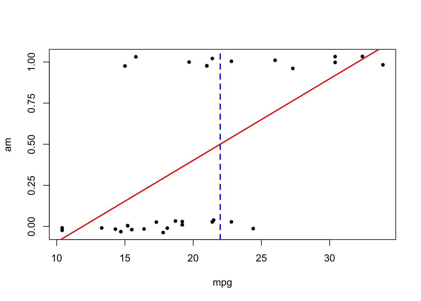
So far we have seen how we can predict quantitative outcomes using regression. But, we can also predict the probability of categorical outcomes occurring, particularly binary outcomes. We can look at an example of this using simple linear regression. Since linear regression only really makes sense to predict quantitative values (it does not make sense to have a transmission type be a decimal value between automatic and manual), we might decide to let it estimate the probability, that is \(P(\text{manual} | X)\), of the car being a manual transmission vehicle (am=1).
# Jitter is done to move the points so they aren't on top of each otherplot(mtcars$mpg, jitter(mtcars$am, .2), pch=20,ylab="am", xlab="mpg", yaxp =c(0, 1, 4))model <-lm(am ~ mpg, data=mtcars)abline(model, col="red", lwd=2)abline(v=21.98, col="blue", lty=2, lwd=2) # Mark at 50%
In the visualization above, we drew a vertical line that equates to the mark where the probability to the right is greater than 0.5 and thus would be classified as a manual transmission. The area to the left would have a probability of less than 0.5 and would be classified as an automatic transmission. There are issues with this approach though, as what would it mean for a car with an mpg of 40 to have the probability of having a manual transmission be 1.39? Or a car with an “mpg” of 5 to have a negative probability of being a manual transmission vehicle? Thinking back to probability theory, the only possible values we can have are between 0 and 1 (inclusive). Therefore, we will need to have a function that is limited to the range \([0,1]\).
7.1 Why Logistic Regression?
While many functions meet this criterion, one function we will use is the logistic function: \[f(x) = \frac{1}{1+e^{-x}} = \frac{e^x}{e^x + 1}\] Using limits we can show that when \(x\) approaches \(\infty\), \(f(x)\) approaches 1 and when \(x\) approaches \(-\infty\), \(f(x)\) approaches 0. When we were using linear regression we were modeling the probabilities as \(p(X) = \beta_0 + \beta_1x_1\). The logistic regression model, a model within the family of Generalized Linear Models (GLM), can then be written as: \[p(X) = \frac{e^{\beta_0 + \beta_1 x_1}}{e^{\beta_0 + \beta_1 x_1} + 1}\] This model is no longer interested in minimizing the Residual Sum of Squares (RSS) but is instead interested in maximizing the likelihood of accurately predicting the probability of 1 occurring. This can be written as \(l(\beta_0, \beta_1) = \prod P(x_i)\cdot \prod (1-P(x_{i'}))\), but it is usually easier to maximize the log-likelihood. This model still retains the linear assumption (the log odds having a linear relationship) and the independence of observations and features. This model does not rely on the residuals to be normally distributed or for there to be a constant variance.
7.2 Odds, Log Odds, and Probability
Doing a little bit of math, we can manipulate the logistic regression model to calculate the odds: \[\frac{p(X)}{1-p(X)} = e^{\beta_0 + \beta_1 x_1}\]
This will result in a value between 0 and \(\infty\) with the larger the value the more likely the probability is to occur (in our case the car being automatic, automatic: \(y=1\)). If the odds are 3 then the probability of the event occurring is 0.75, which we can think of as success 3 times and failure 1 time (giving us \(3/4=0.75)\). Likewise, if the odds are 0.25 (or \(1/4\)), then the probability is 0.20 since we have 1 success and 4 failures (giving us \(1/5=0.2\)).
By taking the logarithm of both sides, we can obtain a formula to calculate the log odds (logit): \[\log \left(\frac{p(X)}{1-p(X)} \right) = \beta_0 + \beta_1 x_1\]
The right-hand side should look familiar to us, as this looks like a linear model. The output in R will calculate the log odds for us, we will then need to calculate the probability from it. The summary of a logistic model will look similar to the linear model, but we will be able to interpret \(\beta_1\) as when we increase \(x_1\) by a one-unit change and hold all other variables constant, the log odds changes by \(\beta_1\).
7.3 Building Logistic Regression Models in R
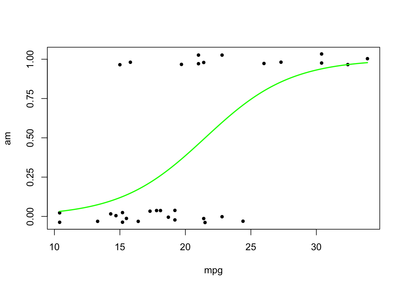
To build the model in R, we can use the glm() function and specify the family as binomial(). We will want to prepare the data before building a model though, as categorical nominal data should be converted to a factor and categorical ordinal data should be converted to quantitative data. Additionally, the outcome should be a quantitative binary response (values 0 and 1) and not a factor. We will not want to keep variables that identify an observation (names, etc.) or any observations with missing values. Visualizing the line of best fit shows the different probabilities for all possible mpg values. We can then plot it similar to how we have in the past when plotting lines in base R. Similar methods are available in ggplot().
Looking at the output below, we can see that all variables are significant. In addition to this, we can see the AIC metric since \(R^2\) will not make sense when dealing with categorical outcomes. The log odds model can be written as: \(-6.6 + 0.307\cdot\text{mpg}\). So, an increase of 1 unit mpg results in a log odds increase of 0.307. The log odds increasing is somewhat difficult to calculate, but whenever \(\beta>0\) it will increase the odds of value 1 occurring, and whenever \(\beta<0\) it will decrease the odds of value 1 occurring.
summary(logistic_model)
Call:
glm(formula = am ~ mpg, family = binomial(), data = mtcars)

Coefficients:
            Estimate Std. Error z value Pr(>|z|)
(Intercept)  -6.6035     2.3514  -2.808  0.00498 **
mpg           0.3070     0.1148   2.673  0.00751 **
---
Signif. codes:  0 '***' 0.001 '**' 0.01 '*' 0.05 '.' 0.1 ' ' 1

(Dispersion parameter for binomial family taken to be 1)

    Null deviance: 43.230  on 31  degrees of freedom
Residual deviance: 29.675  on 30  degrees of freedom
AIC: 33.675

Number of Fisher Scoring iterations: 5
We could also convert the coefficients to odds using the exp() function. The scale has been changed, so now when the value is greater than 1 it indicates the odds of success have increased, and when the odds are less than 1 the odds of success have decreased, holding all other variables constant.
exp(coef(logistic_model)) # odds
(Intercept)         mpg
0.001355579 1.359379288
Below are the different log odds, odds, and probabilities for a few possible mpg values. Using the predict function will probably be the easiest way to carry out these calculations, but it should be done manually as well. When wanting to calculate the probabilities, the argument type=``response" needs to be declared.
predict(logistic_model,df,type="response") # probability
        1         2         3         4
0.1194021 0.3862832 0.7450109 0.9313311
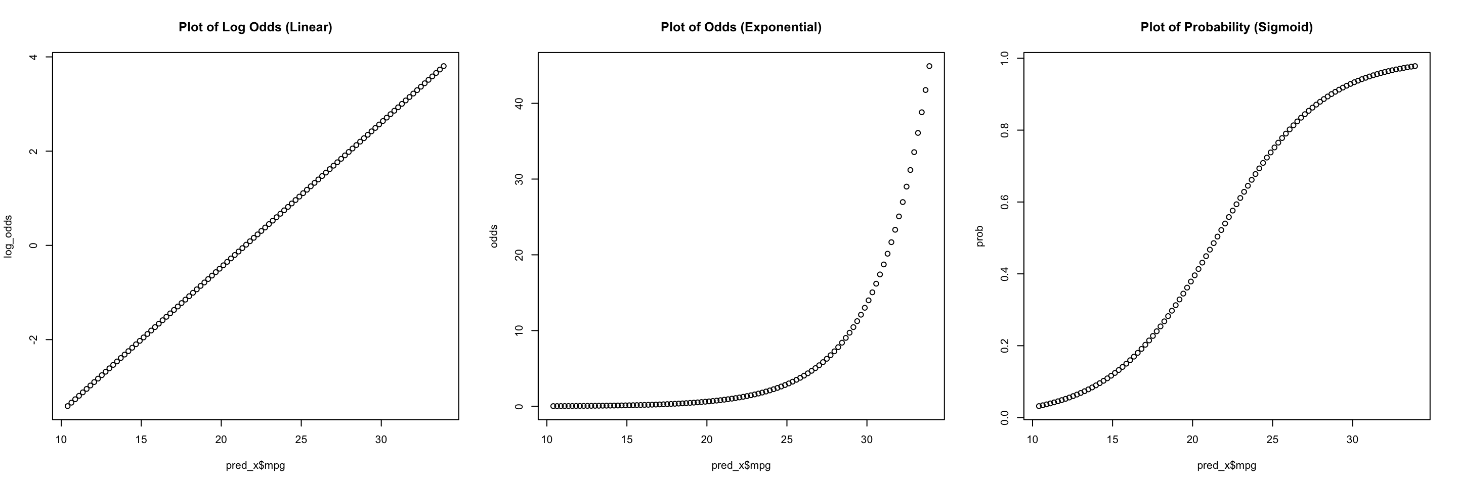
The last thing we will see is how each of the values (log odds, odds, and probability) look when plotted. Notice the shape of each function and how they relate back to their definitions.
#|plot(pred_x$mpg, log_odds, main="Plot of Log Odds (Linear)")plot(pred_x$mpg, odds, main="Plot of Odds (Exponential)")plot(pred_x$mpg, prob, main="Plot of Probability (Sigmoid)")
7.4 Assessing Logistic Regression Models
When looking at a Logistic Regression model, the concept of minimizing the residuals does not apply. This is because when we dealt with linear regression we were predicting outcomes but when we perform logistic regression we are predicting the probability of the observation being in the “positive” class. So instead of trying to minimize the RMSE, logistic regression aims to maximize the likelihood to make the observed data most probable under the model. Essentially the algorithm will adjust the model’s coefficients until the predicted probabilities make the observed outcomes as probable as possible.
To evaluate the model we will need to discuss the idea of deviance. Deviance measures how much the model differs from an ideal model that fits the data perfectly. It can be calculated as \(d_i=-2\times \log(\text{Likelihood})\) where the lower the deviance the better the model. The two types of deviance that we will use to evaluate our model are null deviance and residual deviance. The Null Deviance calculates the deviance of a null model (one with just an intercept) that predicts a constant probability. The residual deviation calculates the deviance of the model with predictors included. The model with the lowest residual deviance will fit the data the best (be cautious of overfitting!). We can see these values when we create a logistic regression model and view the summary:
Call:
glm(formula = Survived ~ ., family = binomial(), data = titanic_1)

Coefficients:
             Estimate Std. Error z value Pr(>|z|)
(Intercept)  4.334201   0.450700   9.617  < 2e-16 ***
Pclass2     -1.414360   0.284727  -4.967 6.78e-07 ***
Pclass3     -2.652618   0.285832  -9.280  < 2e-16 ***
Sexmale     -2.627679   0.214771 -12.235  < 2e-16 ***
Age         -0.044760   0.008225  -5.442 5.27e-08 ***
SibSp       -0.380190   0.121516  -3.129  0.00176 **
---
Signif. codes:  0 '***' 0.001 '**' 0.01 '*' 0.05 '.' 0.1 ' ' 1

(Dispersion parameter for binomial family taken to be 1)

    Null deviance: 964.52  on 713  degrees of freedom
Residual deviance: 636.56  on 708  degrees of freedom
  (177 observations deleted due to missingness)
AIC: 648.56

Number of Fisher Scoring iterations: 5
If we think back to basic probability pertaining to the Binomial distribution, the variance is \(\sigma^2 = n\cdot p \cdot (1-p)\) where \(p\) is the probability of value 1 occurring. We will want to verify the model does not have a larger variance than expected. To do this, we can calculate the dispersion parameter \(\phi\) (pronounced fi) as:
\[\phi = \frac{\text{Residual Deviance}}{\text{Residual Deviance degree of freedom}}\]
If \(\phi\) is much greater than 1 then we have evidence of overdispersion. This will lead to distorted standard errors, inaccurate tests of significance, and inaccurate parameter estimations. If the model exhibits overdispersion then we may look into adding omitted predictors or using a “quasibinomial” distribution to build the model.
While \(R^2\) does not exist for logistic regression, we can calculate a Pseudo-\(R^2\) value by calculating the ratio between the residual and null deviance. It should be noted that this is just an estimate and should not be interpreted in the same way that we interpret \(R^2\) for linear regression models. The calculation can be seen below (if the \(R^2\) results in a value less than 1 then the model is not reliable):
The comparable metric for Adjusted \(R^2\) would be the AIC. The Akaike Information Criterion will reward goodness of fit while penalizing model complexity. We will prefer smaller AIC values between models. But, we should note that the value by itself will not tell us much (much like RMSE), we will need to compare it to other models to see what value is “good”.
log_summary$aic
[1] 648.5646
7.5 Feature Selection
Finally, we can perform feature selection for logistic regression in a similar way we performed it when dealing with linear regression. To do this we will use the anova() function with the argument test="chisq". This will be comparable to forward selection, so you might need to look for which variable results in the largest drop in Deviance and include those first until the others are no longer significant. An example of this can be seen below with a full model. Notice how the AIC is larger than our first model (because this is more complex) while the Residual Deviance is smaller (since we added more features). The anova() function indicates that 4 variables might be the best for our model: