library(ggplot2)
model <- lm(hwy ~ displ, data=mpg)
summary(model)$r.square
[1] 0.5867867plot(mpg$displ, mpg$hwy, pch=20) # pch=20 makes it a solid dot
abline(model, col="red", lwd=2)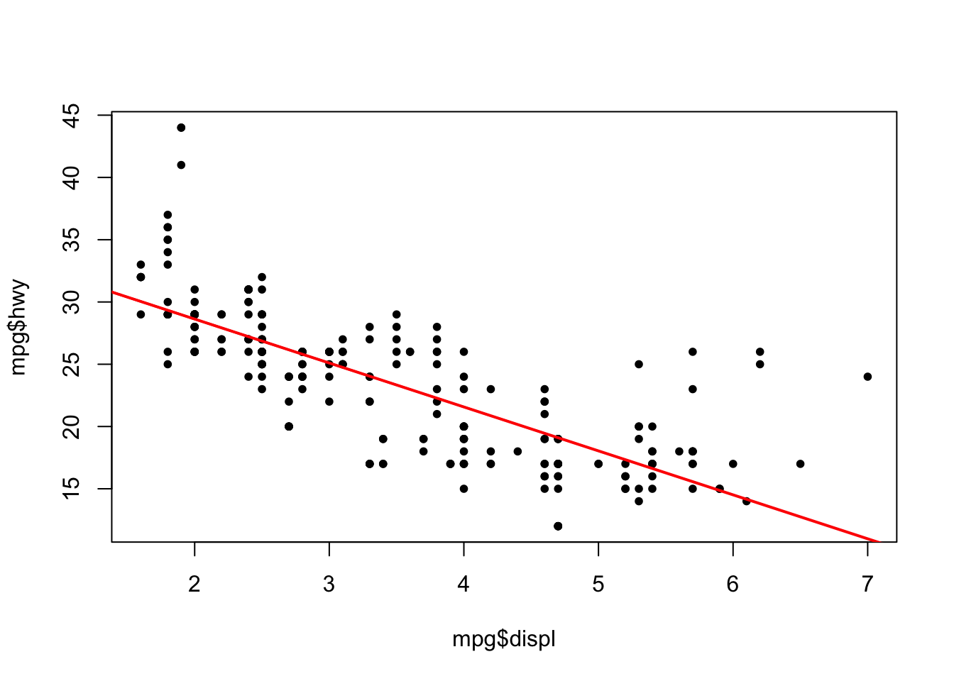
Often when we are looking at a dataset we might notice that a trend is present within categorical features. We can incorporate these categorical features in our Simple Linear Regression (SLR) model with a slight modification to our model. Throughout this lecture, we will be using the ggplot2 library along with some plotting in ggplot. While everything could be done in base R, it is sometimes a hassle to make certain plots. For those who have not experienced ggplot, I will make the code as easy to follow as possible and provide a template for you to use on other questions.
Let us start this lecture by creating a simple linear model that we have seen before using the mpg dataset (inside the ggplot2 library). We can see that the model has a \(R^2\) value of 0.587 which would indicate that it would be decent, but not great, in making predictions and describing the data. We could look at the model in more detail and notice that the coefficients are statistically significant (so we can say they are different than 0), as well as look at the diagnostic plots to confirm a linear model is appropriate for this data.
library(ggplot2)
model <- lm(hwy ~ displ, data=mpg)
summary(model)$r.square[1] 0.5867867plot(mpg$displ, mpg$hwy, pch=20) # pch=20 makes it a solid dot
abline(model, col="red", lwd=2)
If we do some exploratory data analysis, we might detect that the distribution of the hwy variable looks different if we break it apart by model “year” (which can be seen using bow-and-whisker plots). Notice how the medians are slightly different, the IQR, and the skewing are different for the years. We should also notice that “year” makes more sense as a categorical factor then a quantitative value, which can be fixed fairly easily.
mpg$yearf <- factor(mpg$year)
plot(mpg$yearf, mpg$hwy, xlab="year as factor", ylab="hwy mpg")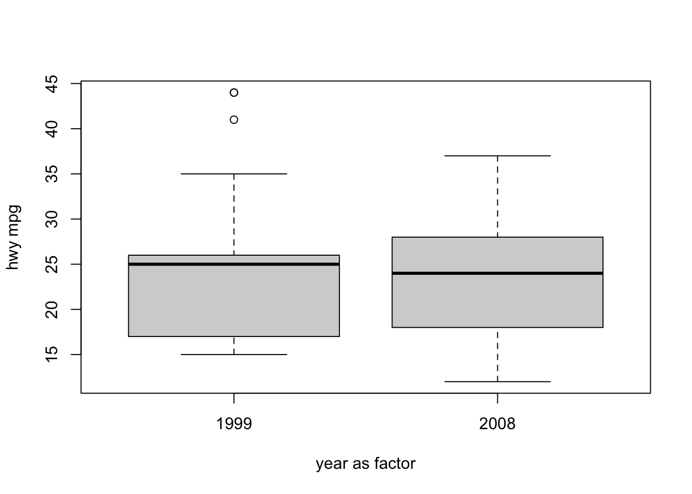
Before incorporating the categorical feature into our model, let’s quickly review our previous model. Our last model looked something like the following:
\[y= \beta_0 + \beta_1 x + \epsilon\] and the new model with the binary categorical feature will be: \[y = \beta_0 + \beta_1x_1 + \beta_2 x_2 + \epsilon\]
Notice how the model incorporates a binary categorical feature. This is because the model can only differentiate if the categorical variable is present. The categories do not necessarily have any intrinsic numeric value. So, to get around this we (R will do it for us) will create a dummy variable which will be 1 when the feature is present and 0 otherwise. This allows us to incorporate a categorical variable with 2 features using only 1 variable. To get a better idea of this, let’s build our model and look at the output:
model <- lm(hwy ~ displ + yearf, data=mpg)
model
Call:
lm(formula = hwy ~ displ + yearf, data = mpg)

Coefficients:
(Intercept)        displ    yearf2008
35.276 -3.611 1.402 Interpreting this model takes a little bit more work since we are dealing with multiple lines. The intercept will tell us the average “hwy” value for 1999 cars when “displ” is 0. The coefficient yearf2008 represents the estimated average change in “hwy” from 1999 to 2008, controlling for other features (everything else held constant). Additionally, “hwy” decreased by 3.31 mpg on average for each unit of change in “displ” regardless of year.
To determine the lines for this model it will help us to write it out. We should note that the variable ``year2008” only equals 1 when looking at cars from 2008. When looking at cars from 1999 the value is 0. Notice how the intercept is the only thing that changes for this model (with the difference determined by the categorical value) and the slope remains the same.
\[\begin{align*} y &= 35.276 - 3.611*\text{displ} + 1.402*\text{yearf2008} \\ \\ \textbf{For 1999 cars: } y&= 35.276 - 3.611*\text{displ} + 1.402*0 \\ y &= 35.276 - 3.611*\text{displ} \\ \\ \textbf{For 2008 cars: } y&= 35.276 - 3.611*\text{displ} + 1.402*1 \\ y &= 36.678 - 3.611*\text{displ} \end{align*}\]
plot(mpg$displ, mpg$hwy, pch=20, col=c("red", "blue")[mpg$yearf])
abline(35.2757, -3.6110, col="red", lwd=2)
abline(35.2757 + 1.4021, -3.6110, col="blue", lwd=2)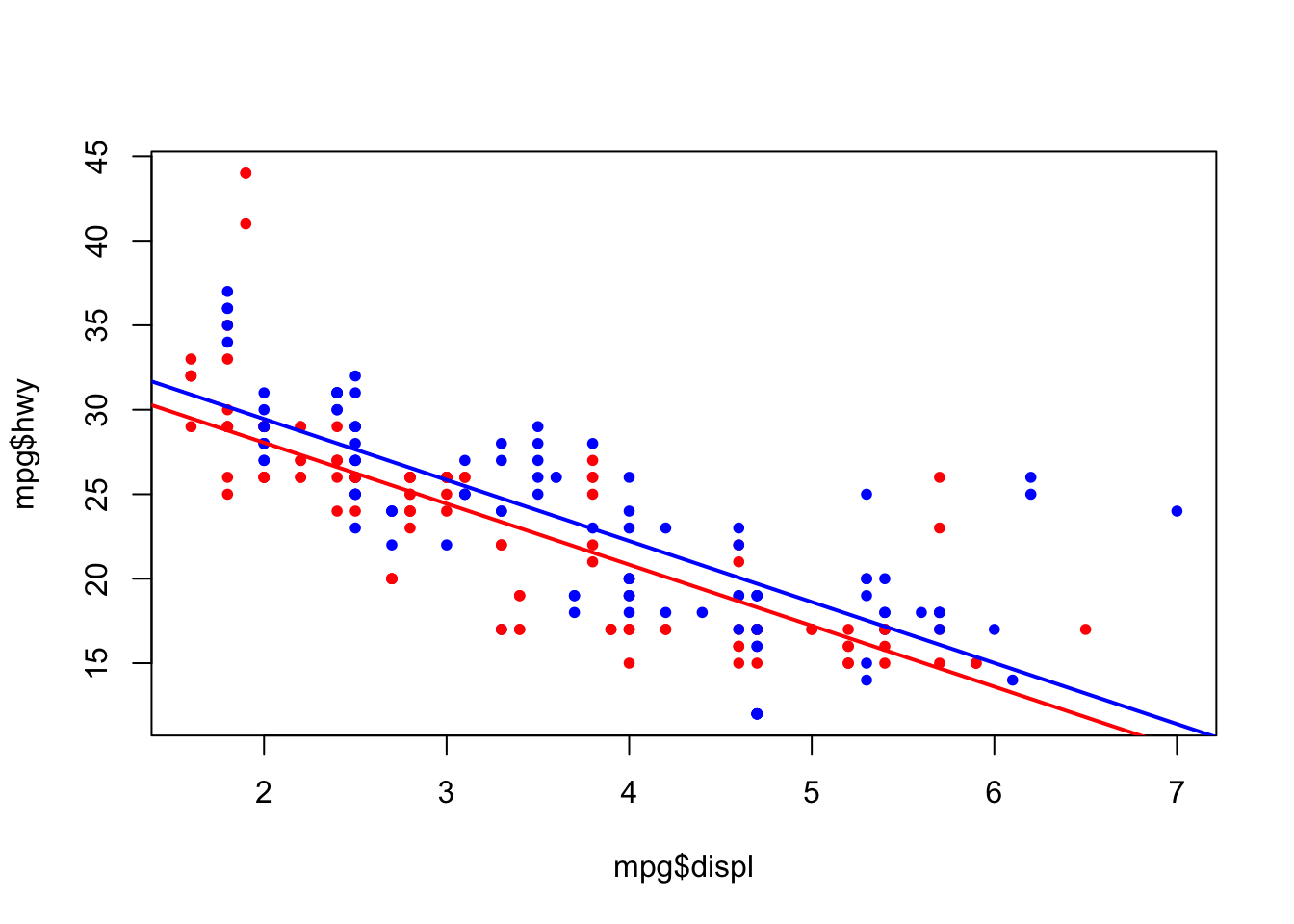
To do this in ggplot we will first need the augment() function within the broom library to quickly determine the fitted values. We can then use them to create our two lines. Within the command, we will tell ggplot the data we are working with and then specify the predictor variable (\(x\)), the outcome variable (\(y\)), and then the categorical variable (\(col\)) inside of the aes() environment. Then we can plot the points using geom_point() and create a line for our model using geom_line(). I will not require you to know how to plot in ggplot, I am just showing you this alternative method in case it is easier for you to do. So, if these commands do not make sense please do not worry.
library(broom)
aug_mod1 <- augment(model)
ggplot(aug_mod1, aes(x=displ, y=hwy, col=yearf)) +
  geom_point() +
  geom_line((aes(y=.fitted)), lwd=1)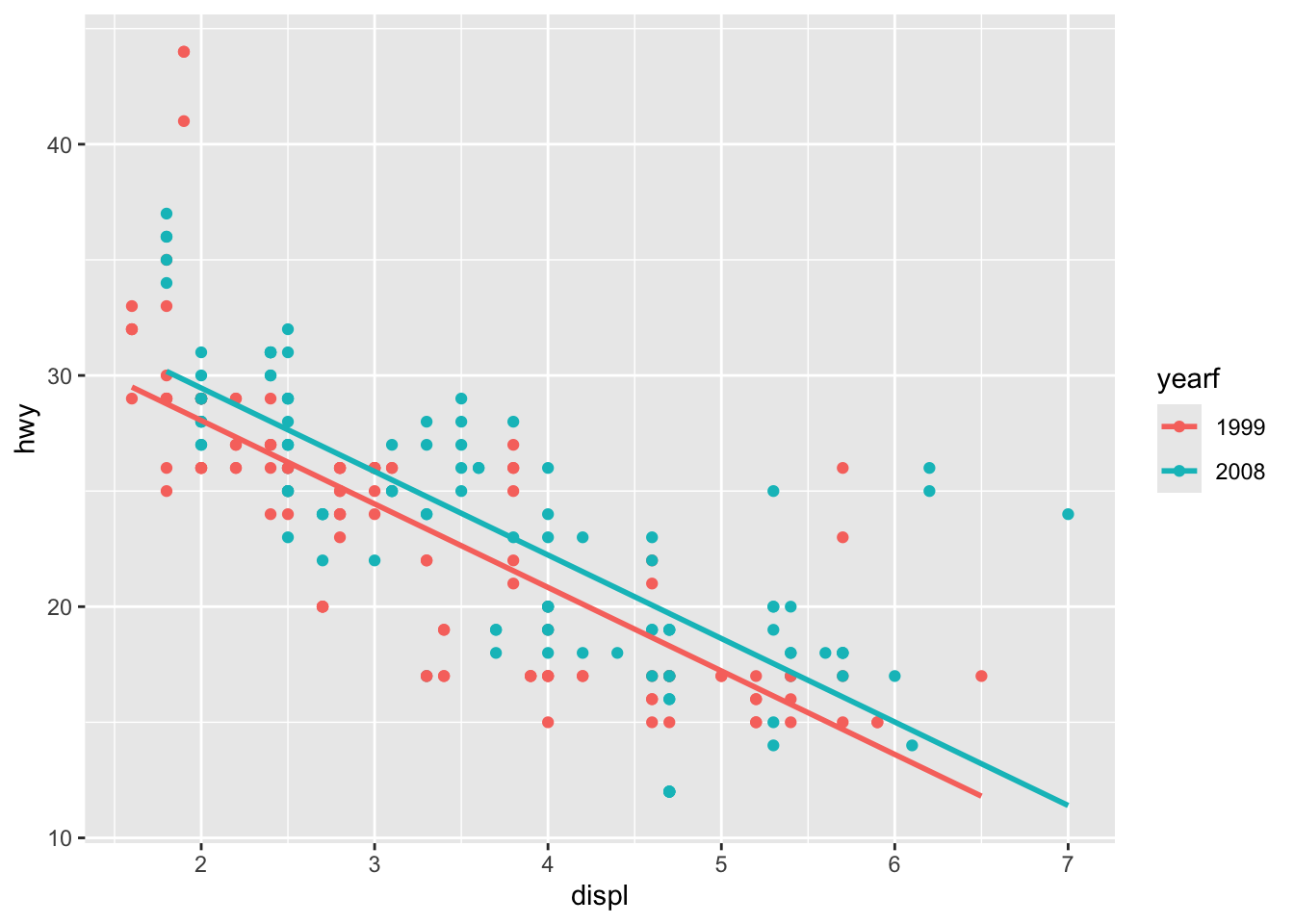
We can take a look at the summary of the model and interpret it (minus the meaning of the coefficients) in a similar way to how we have in the past. We can see that all of the coefficients are statistically significant.
summary(model)
Call:
lm(formula = hwy ~ displ + yearf, data = mpg)

Residuals:
    Min      1Q  Median      3Q     Max
-7.7616 -2.5187 -0.2899  1.8701 15.5852

Coefficients:
            Estimate Std. Error t value Pr(>|t|)
(Intercept)  35.2757     0.7257  48.610  < 2e-16 ***
displ        -3.6110     0.1938 -18.630  < 2e-16 ***
yearf2008     1.4021     0.4998   2.806  0.00545 **
---
Signif. codes:  0 '***' 0.001 '**' 0.01 '*' 0.05 '.' 0.1 ' ' 1

Residual standard error: 3.78 on 231 degrees of freedom
Multiple R-squared:  0.6004,    Adjusted R-squared:  0.5969
F-statistic: 173.5 on 2 and 231 DF,  p-value: < 2.2e-16
We can note that the \(R^2\) value is slightly higher for this model than the original model (0.600 vs. 0.587). This is because as we add variables to the model, the \(R^2\) value will always increase. To combat over-fitting our data, we will introduce the concept of parsimony. This will penalize more features being added to the model. The Adjusted \(R^2\) value will now be the metric we will want to look at when calculating how well the model describes the data when we have 2 or more features. The formula for Adjusted \(R^2\) will be:
\[\text{Adjusted }R^2 = 1 - \frac{(1-R^2)(n-1)}{n-p-1}\]
where \(n\) is the number of observations and \(p\) is the number of features. When looking at the summary above, we can see the Adjusted \(R^2\) value is slightly lower than the \(R^2\) value, but it is higher than the original model.
n <- length(mpg$displ)
adj_r2 <- 1 - (1-0.6004)*(n-1)/(n-2-1)
adj_r2
[1] 0.5969403We will now quickly look at an additional problem using the iris dataset. Within this dataset, the Species variable has 3 different possible values. We will first look at a basic simple linear regression model just using Sepal.Length and Sepal.Width. We can see that the model does not do a good job of explaining the variation in our data due to the low \(R^2\) value. It also appears that the Sepal.Length is not correlated with the Sepal.Width at all.
model <- lm(Sepal.Width ~ Sepal.Length, data=iris)
summary(model)
Call:
lm(formula = Sepal.Width ~ Sepal.Length, data = iris)

Residuals:
    Min      1Q  Median      3Q     Max
-1.1095 -0.2454 -0.0167  0.2763  1.3338

Coefficients:
             Estimate Std. Error t value Pr(>|t|)
(Intercept)   3.41895    0.25356   13.48   <2e-16 ***
Sepal.Length -0.06188    0.04297   -1.44    0.152
---
Signif. codes:  0 '***' 0.001 '**' 0.01 '*' 0.05 '.' 0.1 ' ' 1

Residual standard error: 0.4343 on 148 degrees of freedom
Multiple R-squared:  0.01382,   Adjusted R-squared:  0.007159
F-statistic: 2.074 on 1 and 148 DF, p-value: 0.1519plot(iris$Sepal.Length, iris$Sepal.Width, pch=20)
abline(model, col="red", lwd=2)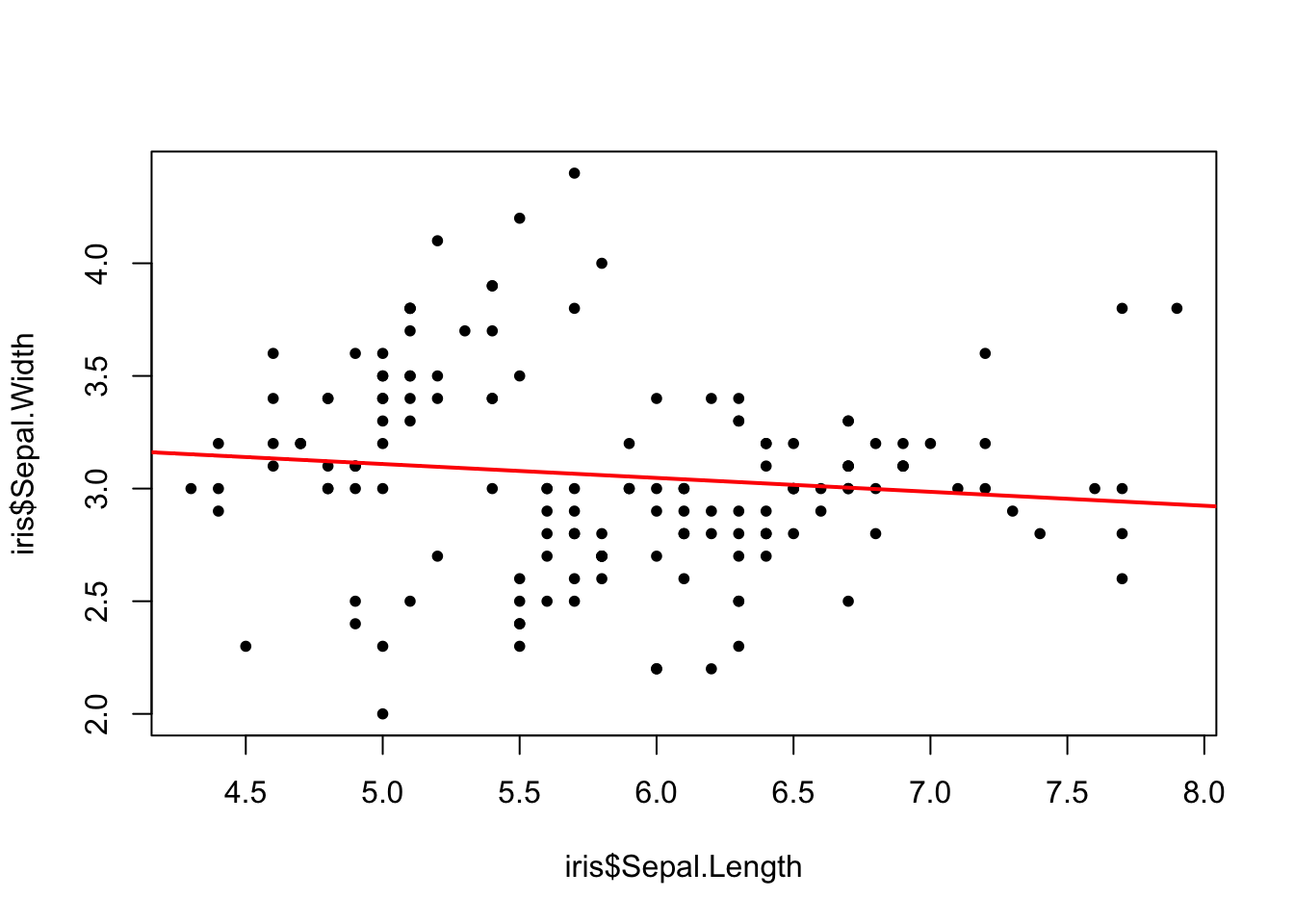
But, if we look more into the data we can see that the distribution of Sepal.Width is different for each Species type. Looking at the box-and-whisker plot, we can easily see the difference in the median between the three Species.
plot(iris$Species, iris$Sepal.Width)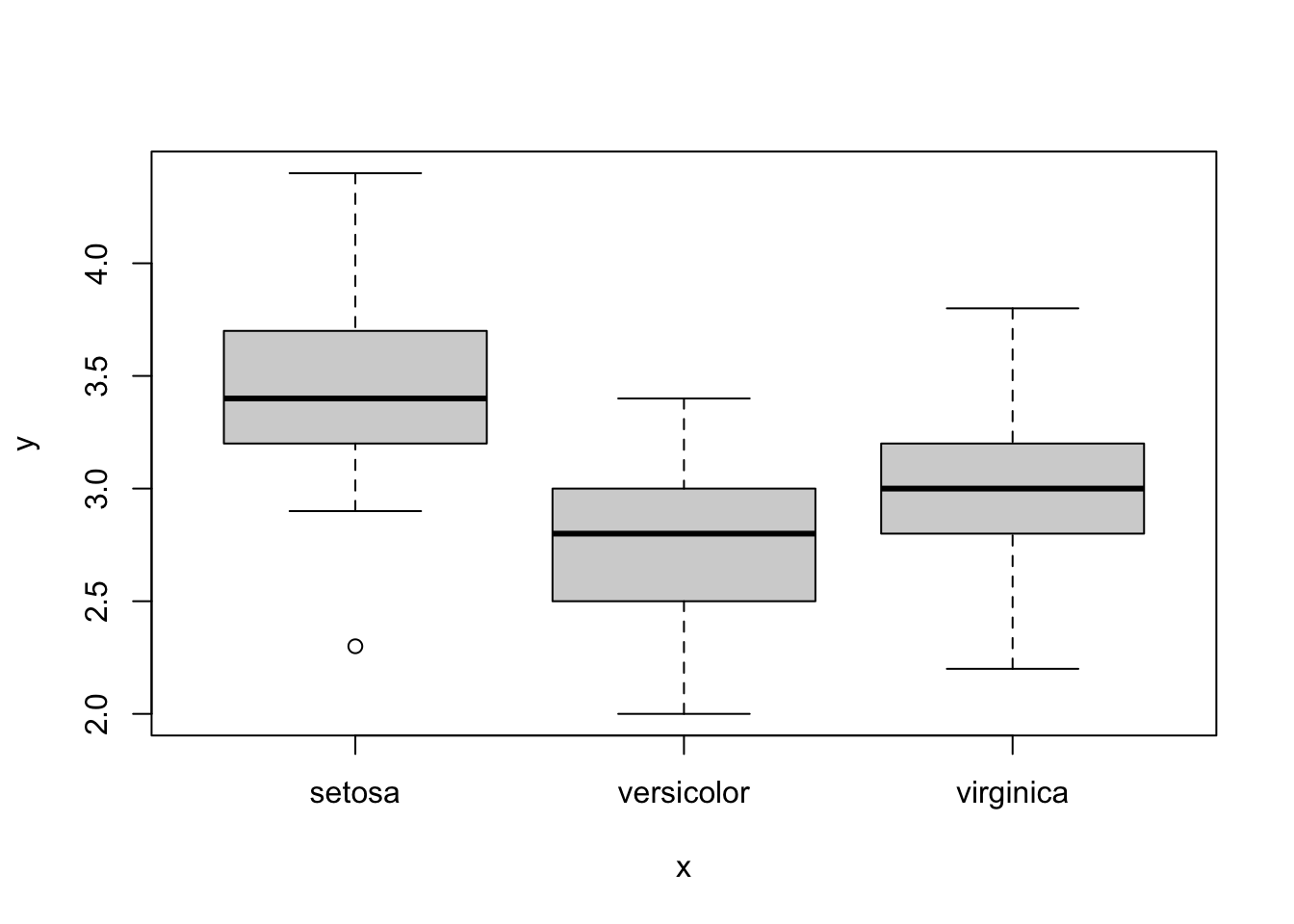
Before building our model with the categorical variable, we are going to reorder the levels within the dataset to make it a little more “exciting” for us. We did this so that one categorical level turns out to not be statistically significant. You can run the model without making this change and see how the output looks different (but will give us the same lines).
iris_ex <- iris
iris_ex$Species <- factor(iris_ex$Species,
                          levels=c("versicolor", "virginica", "setosa"))
Notice how when we have 3 categorical levels we use 2 dummy variables (so they are all “off” or one is “on” at a time). We can calculate the different models as follows:
\[y = 0.69311 + 0.34988*\text{Sepal.Length} - 0.02412*\text{virginica} + 0.98339*\text{setosa}\] \[\begin{align*} \textbf{Versicolor Model: } y&= 0.69311 + 0.34988*\text{Sepal.Length} - 0.02412*0 + 0.98339*0 \\ y &= 0.69311 + 0.34988*\text{Sepal.Length}\\ \\ \textbf{Virginica Model: } y&= 0.69311 + 0.34988*\text{Sepal.Length} - 0.02412*1 + 0.98339*0 \\ y &= 0.66899 + 0.34988*\text{Sepal.Length} \\ \\ \textbf{Setosa Model: } y&= 0.69311 + 0.34988*\text{Sepal.Length} - 0.02412*0 + 0.98339*1 \\ y &= 1.67650 + 0.34988*\text{Sepal.Length} \end{align*}\]
plot(iris_ex$Sepal.Length, iris_ex$Sepal.Width, pch=20,
     col=c("red", "blue", "green")[iris_ex$Species])
abline(0.69311, 0.34988, col="red", lwd=2)
abline(0.69311 - 0.02412, 0.34988, col="blue", lwd=2)
abline(0.69311 + 0.98339, 0.34988, col="green", lwd=2)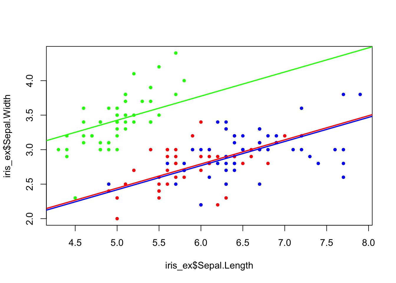
summary(model)
Call:
lm(formula = Sepal.Width ~ Sepal.Length, data = iris)

Residuals:
    Min      1Q  Median      3Q     Max
-1.1095 -0.2454 -0.0167  0.2763  1.3338

Coefficients:
             Estimate Std. Error t value Pr(>|t|)
(Intercept)   3.41895    0.25356   13.48   <2e-16 ***
Sepal.Length -0.06188    0.04297   -1.44    0.152
---
Signif. codes:  0 '***' 0.001 '**' 0.01 '*' 0.05 '.' 0.1 ' ' 1

Residual standard error: 0.4343 on 148 degrees of freedom
Multiple R-squared:  0.01382,   Adjusted R-squared:  0.007159
F-statistic: 2.074 on 1 and 148 DF,  p-value: 0.1519
We can see based on the summary of the model that not all levels are statistically significant. That means with this model the Virginica species intercept is not statistically different than the Versicolor species. But, as long as one level is statistically significant we will retain the full categorical feature. Also, notice that the Adjusted \(R^2\) value of the model including the categorical variables Species is better than when the variable is not present (0.560 vs. 0.014).
It should be mentioned that we should only build models and interpret results like this when we are dealing with unordered factors (nominal data). Dealing with Ordinal data is a much more complicated concept, one that we could spend a whole semester on alone.
If we remember, the categorical coefficients only impacted the intercept, as all of the lines had parallel slope. This means that the slope for the prediction variable was not impacted by the categorical factor. In our case, displ was not impacted by year. But, it would probably make sense that displ could vary by year (that is the slope of the lines differ based on the year).
To implement this, we will need to introduce the idea of interactions between features. Here the relationship between one feature and outcome depends on the level of another feature. This will allow us to account for the interaction between features. To understand how we will do this in our model, let’s look at the equation for a simple linear model, a model with a categorical factor, and then finally a model with an interaction term. We will notice that the coefficient \(\beta_3\) has both \(x_1\) (predictor) and \(x_2\) (categorical factor) present:
\[\begin{align*} \textbf{Basic Model: }y&= \beta_0 + \beta_1 x + \epsilon \\ \textbf{Model with Categorical Feature: }y& = \beta_0 + \beta_1 x_1 + \beta_2 x_2 + \epsilon \\ \textbf{Model with Interaction Term: }y& = \beta_0 + \beta_1 x_1 + \beta_2 x_2 + \beta_3 x_1 x_2 + \epsilon \end{align*}\]
If we look at the model above, we can see that \(\beta_2x_2\) will alter the intercept and \(\beta_3 x_1 x_2\) will alter the slope, as \(x_2\) will either be 0 or 1. The model could be expanded to allow for a categorical level with additional features. The “math” to figure out all of the linear equations is shown below. Building the model in R will be exactly the same, except for now we will use a colon to specify the variables which might be interacting with each other.
mpg$yearf <- factor(mpg$year)
model <- lm(hwy ~ displ + yearf + displ:yearf, data=mpg)
model
Call:
lm(formula = hwy ~ displ + yearf + displ:yearf, data = mpg)

Coefficients:
    (Intercept)            displ        yearf2008  displ:yearf2008
        35.7922          -3.7684           0.3445           0.3052
In order to interpret the model, it will help to write it out. Remember that ``yearf2008” equals 1 only when we are looking at the cars from 2008. Notice how in this case both the slope and coefficient are different between models (math shown below): \[\begin{align*} \textbf{General Model:} \\ y &= \beta_0 + \beta_1 \cdot \text{displ} + \beta_2 \cdot \text{yearf2008} + \beta_3 \cdot\text{displ}\cdot\text{yearf2008} \\ \\ \textbf{For 1999 cars:} \\ y &= 35.7922 - 3.7684 \cdot \text{displ} + 0.3445 \cdot 0 + 0.3052 \cdot\text{displ}\cdot0 \\ y &= 35.7922 - 3.7684 \cdot \text{displ} \\ \\ \textbf{For 2008 cars:} \\ y &= 35.7922 - 3.7684 \cdot \text{displ} + 0.3445 \cdot 1 + 0.3052 \cdot\text{displ}\cdot1 \\ y &= (35.7922 + 0.3445) + (-3.7684 + 0.3052) \cdot\text{displ} \\ y &= 36.1367 -3.4632 \cdot\text{displ} \end{align*}\]
plot(mpg$displ, mpg$hwy, pch=20, col=c("red", "blue")[mpg$yearf])
abline(a=35.7922, b= -3.7674, col="red", lwd=2)
abline(a=35.7922 + 0.3445, b= -3.7684+0.3052, col="blue", lwd=2) 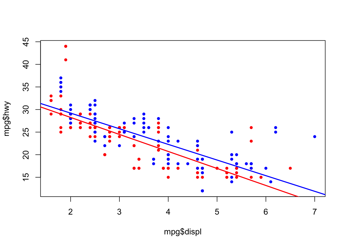
If we remember back to the previous lecture, both lines were parallel and only differed with their intercept value. For this visualization, we can see that the displ variable affects the hwy outcome slightly differently based on the year factor.
We can look at the summary of the model and interpret it in a similar way to how we have been. Looking at the coefficients, it appears that only the intercept and the slope are statistically significant. For this model, neither the categorical factor nor the interaction term are statistically significant. This means that we do not think they are necessarily helpful in explaining our model. Note though that the categorical factor was significant when we did not have the interaction term present. Also note that the \(R^2\) value increased (as it always will when we add more terms to the model) but the Adjusted \(R^2\) dropped slightly compared the the Adjusted \(R^2\) of the model in the previous lecture. Because of this, we might decide to drop the interaction term since it does not add much to the model (and we will always prefer a simpler model to a more complex model if possible).
summary(model)
Call:
lm(formula = hwy ~ displ + yearf + displ:yearf, data = mpg)

Residuals:
    Min      1Q  Median      3Q     Max
-7.8595 -2.4360 -0.2103  1.6037 15.3677

Coefficients:
                Estimate Std. Error t value Pr(>|t|)
(Intercept)      35.7922     0.9794  36.546   <2e-16 ***
displ            -3.7684     0.2788 -13.517   <2e-16 ***
yearf2008         0.3445     1.4353   0.240    0.811
displ:yearf2008   0.3052     0.3882   0.786    0.433
---
Signif. codes:  0 '***' 0.001 '**' 0.01 '*' 0.05 '.' 0.1 ' ' 1

Residual standard error: 3.784 on 230 degrees of freedom
Multiple R-squared:  0.6015,    Adjusted R-squared:  0.5963
F-statistic: 115.7 on 3 and 230 DF,  p-value: < 2.2e-16
Let’s now take a look at the iris dataset and build a similar model to the one we did in the previous lecture. Only now, we will include the interaction term to see if the relationship between Sepal.Length and Sepal.Width is affected by the Species type.
iris_ex <- iris
iris_ex$Species <- factor(iris_ex$Species,
                          levels=c("versicolor", "virginica", "setosa"))
model <- lm(Sepal.Width ~ Sepal.Length + Species + Sepal.Length:Species,
            data=iris_ex)
model
Call:
lm(formula = Sepal.Width ~ Sepal.Length + Species + Sepal.Length:Species,
    data = iris_ex)

Coefficients:
                  (Intercept)                   Sepal.Length
                      0.87215                        0.31972
             Speciesvirginica                  Speciessetosa
                      0.57416                       -1.44158
Sepal.Length:Speciesvirginica     Sepal.Length:Speciessetosa
                     -0.08783                        0.47881
Below we can see how we can determine the equations for all three Species levels. I am abbreviating Sepal.Length as SL for space reasons: \[\begin{align*}
&\textbf{General Model:} \\
&y = \beta_0 + \beta_1 \cdot \text{SL} + \beta_2 \cdot \text{virginica} + \beta_3 \cdot\text{setosa} + \beta_4 \cdot \text{SL} \cdot \text{virginica} + \beta_5 \cdot \text{SL} \cdot \text{setosa} \\ \\
&\textbf{Versicolor Model:} \\
&y = \beta_0 + \beta_1 \cdot \text{SL} + \beta_2 \cdot 0 + \beta_3 \cdot 0 + \beta_4 \cdot \text{SL} \cdot 0 + \beta_5 \cdot \text{SL} \cdot 0 \\
&y = \beta_0 + \beta_1 \cdot \text{SL} \\
&y = 0.87215 + 0.31972 \cdot \text{SL} \\ \\
&\textbf{Virginica Model:} \\
&y = \beta_0 + \beta_1 \cdot \text{SL} + \beta_2 \cdot 1 + \beta_3 \cdot 0 + \beta_4 \cdot \text{SL} \cdot 1 + \beta_5 \cdot \text{SL} \cdot 0 \\
&y = \beta_0 + \beta_1 \cdot \text{SL} + \beta_2 + \beta_4 \cdot \text{SL} \\
&y = (\beta_0 + \beta_2) + (\beta_1 + \beta_4) \cdot \text{SL} \\
&y = (0.87215 + 0.57416) + (0.31972 - 0.08783) \cdot \text{SL} \\
&y = 1.44631 + 0.23189 \cdot \text{SL} \\ \\
&\textbf{Setosa Model:} \\
&y = \beta_0 + \beta_1 \cdot \text{SL} + \beta_2 \cdot 0 + \beta_3 \cdot 1 + \beta_4 \cdot \text{SL} \cdot 0 + \beta_5 \cdot \text{SL} \cdot 1 \\
&y = \beta_0 + \beta_1 \cdot \text{SL} + \beta_3 + \beta_5 \cdot \text{SL} \\
&y = (\beta_0 + \beta_3) + (\beta_1 + \beta_5) \cdot \text{SL} \\
&y = (0.87215 - 1.44158) + (0.31972 + .47881) \cdot \text{SL} \\
&y = -0.56943 + 0.79853 \cdot \text{SL}
\end{align*}\]
plot(iris_ex$Sepal.Length, iris_ex$Sepal.Width, pch=20,
     col=c("red", "blue", "green")[iris_ex$Species])
abline(a= 0.87215, b=0.31972, col="red", lwd=2)
abline(a= 0.87215 + 0.57416, b=0.31972 -0.08783, col="blue", lwd=2)
abline(a= 0.87215 - 1.44158, b=0.31972 + 0.47881, col="green", lwd=2)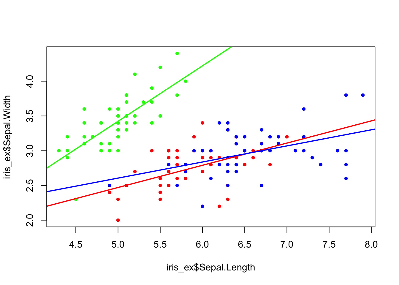
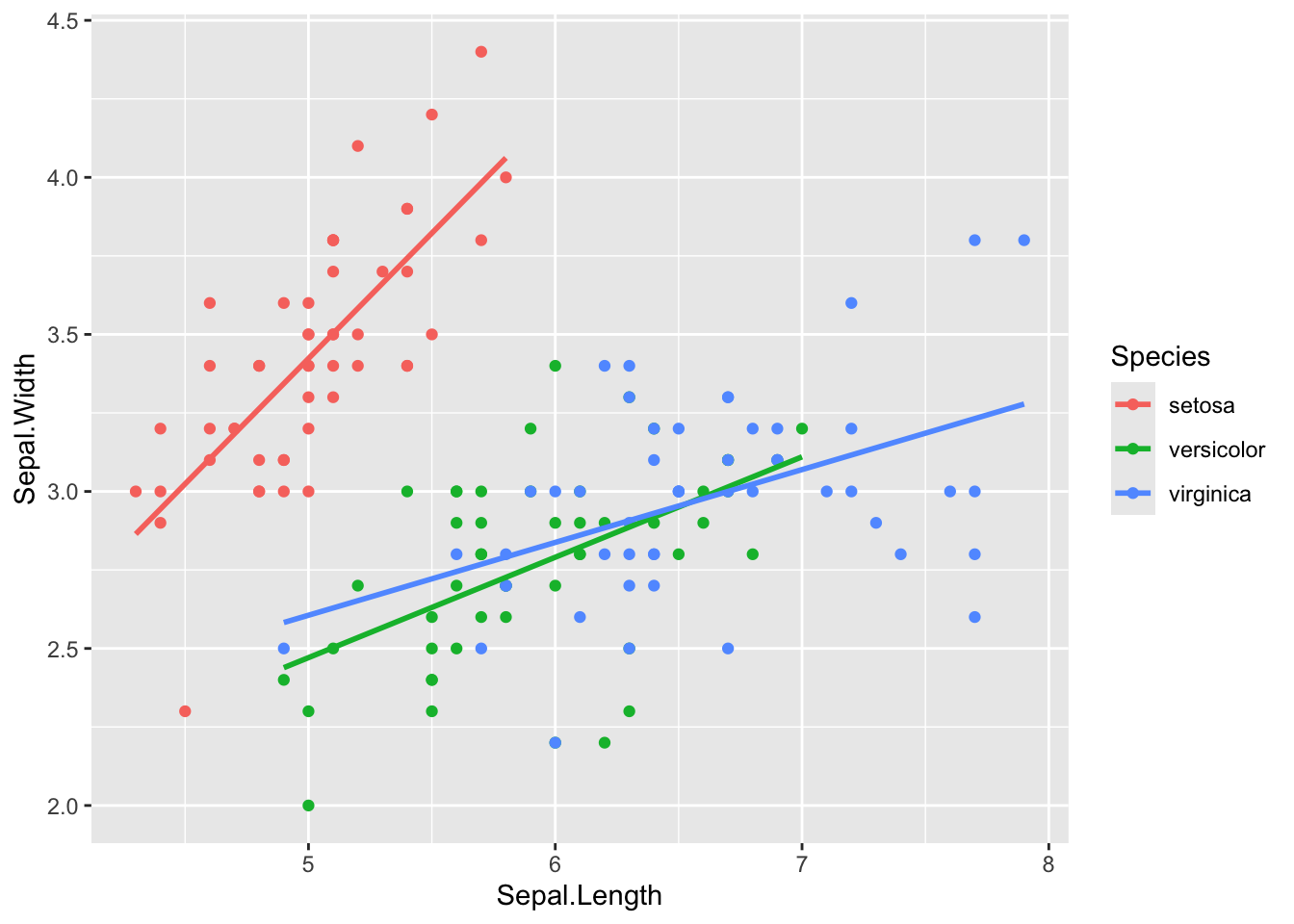
Looking at the visualization above, we can see that the Sepal.Length and Sepal.Width have different relationships between the two variables depending on the Species type. Looking at the summary below, we can see that one of the interaction terms is highly significant (meaning we should probably keep this term in our model). Additionally, a categorical factor term is also significant. If it was not significant then we would still want to keep it since the interaction term is significant. Also, we can notice that this model has a slightly higher Adjusted \(R^2\) value than our model without the interaction term.
summary(model)
Call:
lm(formula = Sepal.Width ~ Sepal.Length + Species + Sepal.Length:Species,
    data = iris_ex)

Residuals:
     Min       1Q   Median       3Q      Max
-0.72394 -0.16327 -0.00289  0.16457  0.60954

Coefficients:
                              Estimate Std. Error t value Pr(>|t|)
(Intercept)                    0.87215    0.44906   1.942 0.054072 .
Sepal.Length                   0.31972    0.07537   4.242 3.95e-05 ***
Speciesvirginica               0.57416    0.60466   0.950 0.343926
Speciessetosa                 -1.44158    0.71304  -2.022 0.045056 *
Sepal.Length:Speciesvirginica -0.08783    0.09708  -0.905 0.367128
Sepal.Length:Speciessetosa     0.47881    0.13365   3.582 0.000465 ***
---
Signif. codes:  0 '***' 0.001 '**' 0.01 '*' 0.05 '.' 0.1 ' ' 1

Residual standard error: 0.2723 on 144 degrees of freedom
Multiple R-squared:  0.6227,    Adjusted R-squared:  0.6096
F-statistic: 47.53 on 5 and 144 DF,  p-value: < 2.2e-16
Below we can see how both plots can be replicated in ggplot. Note that it only plots the linear model (with interactions) for us, it does not specify what the model is. To understand the model, we will need to know how to interpret the results of the summary (and calculate the equation ourselves!).
ggplot(mpg, aes(x=displ, y=hwy, col=yearf)) +
  geom_point() +
  geom_smooth(method="lm", se=FALSE)
`geom_smooth()` using formula = 'y ~ x'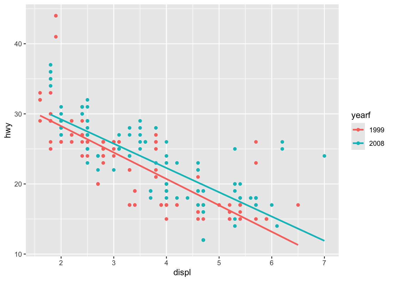
ggplot(iris, aes(x=Sepal.Length, y=Sepal.Width, col=Species)) +
  geom_point() +
  geom_smooth(method="lm", se=FALSE)
`geom_smooth()` using formula = 'y ~ x'