In the previous lecture, we saw how we could build decision trees for classification purposes. In this lecture, we will look into building decision trees for regression purposes. We have performed regression previously using simple linear, multiple linear, and even polynomial/transformed models where we try to predict the quantitative outcome value. We can do the same using decision trees, with all observations in a given category being assigned the same predicted value.
12.1 Regression Trees and RSS
Instead of making the binary splits based on the information gained and trying to make homogeneous groups, we will aim to select the split that results in the lowest RSS. Remember that RSS is the Residual Sum of Squares and \(\hat{y}\) is the predicted outcome value found by averaging the outcome values of all of the observations in the same split: \[\textit{RSS}=\sum{(\hat{y} - y_i)^2}\]
This is a similar metric (although slightly different) that we used when determining which linear regression line was closest to our outcome values. So, when we make a decision tree we are looking for the split which minimizes the total residual sum of squares: \[RSS_\text{split} = RSS_\text{node 1} + RSS_\text{node 2}\]
This machine learning model is a top-down greedy algorithm, meaning that we start with a single grouping of data and successively split the data using the best split at that specific moment (as opposed to looking ahead and determining if a different split will lead to a better future tree).
12.2 Building Regression Trees in R
We can perform this in R fairly easily using the same code we used when dealing with classification decision trees. To see this example, we will look at the Hitters data in the ISLR library. We will aim to predict the salary of baseball players using only a few predictor variables:
library(ISLR)library(tree)Hitter_tree <-tree(Salary ~ Hits + Years + CHmRun, data=Hitters)summary(Hitter_tree)
Regression tree:
tree(formula = Salary ~ Hits + Years + CHmRun, data = Hitters)
Number of terminal nodes:  9
Residual mean deviance:  75300 = 19130000 / 254
Distribution of residuals:
    Min.  1st Qu.   Median     Mean  3rd Qu.     Max.
-1057.00  -128.20   -27.36     0.00   100.20  1451.00
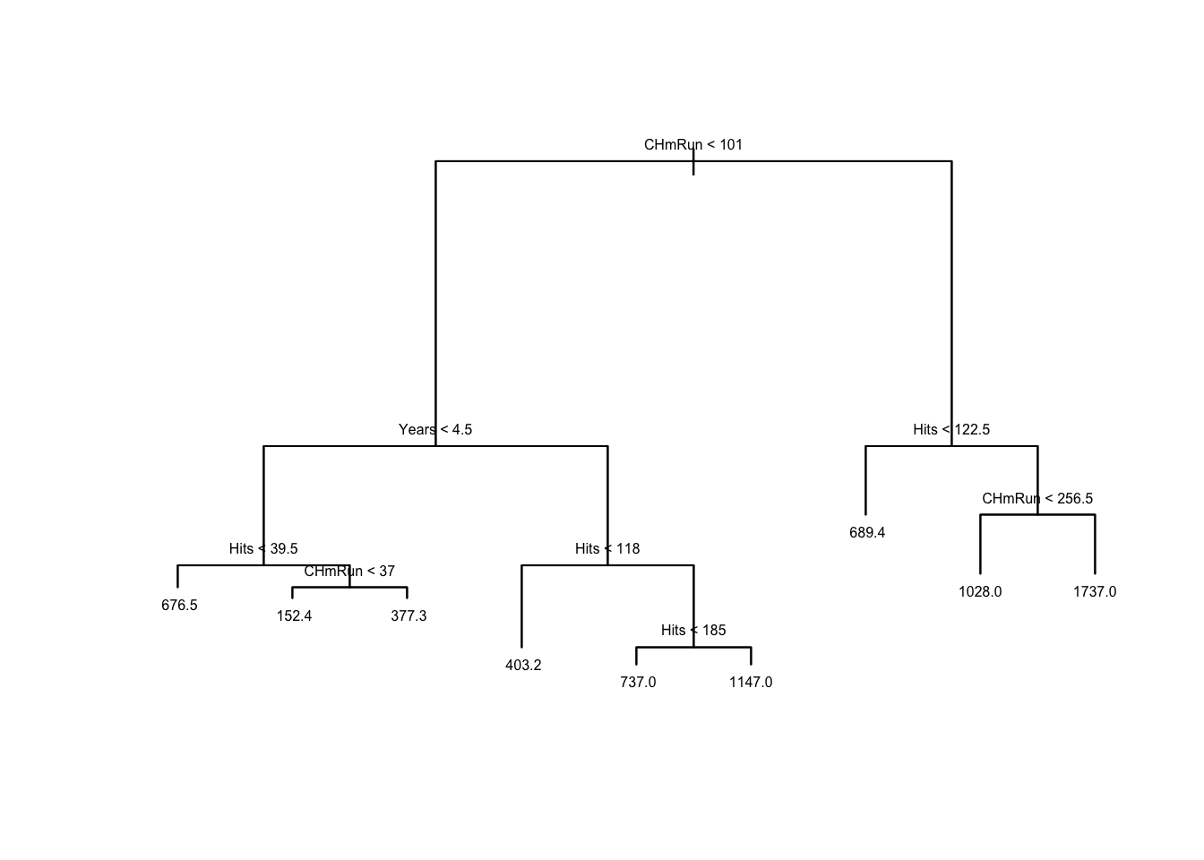
Looking at the summary above, we can see that a decision tree with 9 nodes has been created in order to predict the average salary a player would have given their previous year’s Hits total, the number of Years in the League they have played, and the Career number of HomeRuns. The residual mean deviance describes the average squared difference between the observed and predicted values within the nodes. A plot of the decision tree can be found below:
plot(Hitter_tree)text(Hitter_tree, cex=0.5)
Looking at the decision tree above, we can see that the number one factor in determining the salary of a baseball player is the Career number of HomeRuns they have hit. If they have hit more than 101 home runs and had less than 122.5 hits last year their predicted salary would be 689.4. If they had more than 122.5 hits but less than 256.5 Career HomeRuns then their salary would be 1028 on average and if they had more than 256.5 Career HomeRuns then their salary would be 1737 on average. The same determination could be made with the left-hand side of the tree.
12.3 Evaluating Regression Trees
Let’s also take a look at the College dataset in the ISLR library. We want to try to predict the cost of out-of-state tuition. We are going to split the data into a training and testing group, see how well our predictions are, and then prune the tree and see how the predictions change. Pruning the tree is important as a large complex tree might overfit the training data and lead to high bias and low variance while too basic of a tree will not capture the general trend of the data and result in low bias and high variance:
Regression tree:
tree(formula = Outstate ~ ., data = train)
Variables actually used in tree construction:
[1] "Expend"      "Private"     "Apps"        "Room.Board"  "perc.alumni"
[6] "Grad.Rate"   "Terminal"
Number of terminal nodes:  12
Residual mean deviance:  3309000 = 1.886e+09 / 570
Distribution of residuals:
     Min.   1st Qu.    Median      Mean   3rd Qu.      Max.
-6613.000 -1087.000    -4.945     0.000  1094.000  6596.000
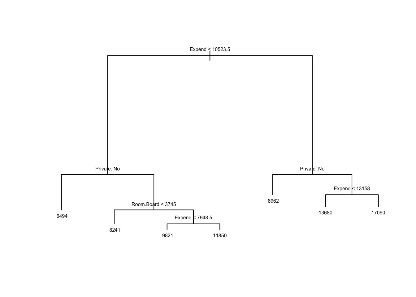
Looking at the summary and decision tree above, we can see that 7 predictor variables go into making the 12 terminal node model with the residuals being fairly symmetric. We can calculate the Testing RMSE on this decision tree before we prune the tree:
predicted_values <-predict(College_tree, newdata=test)sqrt(mean((predicted_values - test$Outstate)^2)) # Test RMSE
[1] 2048.109
12.4 Pruning Regression Trees
We might decide that we wish to prune the tree to make it simpler. For instance, maybe we think it is too complicated to explain the model with 12 terminal nodes and we wish to reduce it, or we wish to avoid overfitting. To prune the tree we can use cross-validation, using the cv.tree() function, to determine the ideal number of nodes for the tree to have. We will select the one with the lowest “dev”. In our example, the 12-node model is the ideal one, but let’s run through the code to make the model a 7-node decision tree as an example.
Regression tree:
snip.tree(tree = College_tree, nodes = c(6L, 15L, 10L, 4L, 14L
))
Variables actually used in tree construction:
[1] "Expend"     "Private"    "Room.Board"
Number of terminal nodes:  7
Residual mean deviance:  4343000 = 2.497e+09 / 575
Distribution of residuals:
    Min.  1st Qu.   Median     Mean  3rd Qu.     Max.
-8448.00 -1241.00    55.52     0.00  1350.00  6770.00