In previous lectures, we have seen how we can build a simple linear model using a quantitative predictor variable. We also saw how we can expand that idea and add multi-level categorical features, including interaction terms, to the model. We are going to continue to expand on this idea by now adding more quantitative features to the model. Adding additional quantitative predictor variables to the model will make it harder (if not impossible) to visualize, so knowing how to interpret the model will be extremely important.
where \(n\) is the number of features. The goals of this model will remain the same as they have been: minimize the RMSE. Additionally, the assumptions will also remain the same; having a linear relationship, having the residuals be normally distributed, having the observations be independent from one another, and having a constant variance. It may be hard to visualize all of these assumptions by just looking at the data, but reading the diagnostic plots will help us tremendously.
4.1 Building a Multiple Linear Regression Model
Building the model in R will be exactly the same as how we have done it before. We will just specify multiple predictor variables by adding a \(+\) to the model. If we want to include all variables from the dataset (except for the outcome variable) as predictor variables then after the tilde we would put a “\(.\)” (period). We should be careful with this though as it will include all categorical features as well, which may make it hard to interpret. If we want to exclude a certain feature then we can do so with the minus sign “\(-\)”.
To see this process played out, we can look at the states.x77 dataset. The code below turns it into a dataframe and only selects certain variables to be in the newly created dataset called states. A linear model is then built using the variables Population, Illiteracy, Income, and Frost to predict the Murder rate in each state.
states <-as.data.frame(state.x77[,c("Murder", "Population","Illiteracy", "Income", "Frost")])model1 <-lm(Murder ~ ., states)model1
Call:
lm(formula = Murder ~ ., data = states)

Coefficients:
(Intercept)   Population   Illiteracy       Income        Frost
  1.235e+00    2.237e-04    4.143e+00    6.442e-05    5.813e-04
We can also look at the summary of the model and notice that only 2 variables are statistically significant (meaning we have evidence to say they are different than 0). We can also see that the Adjusted \(R^2\) tells us the model accounts for roughly \(53\%\) of the variation in the data. Looking at the \(F\)-statistic, it appears the overall model is significant due to its small \(p\)-value.
summary(model1)
Call:
lm(formula = Murder ~ ., data = states)

Residuals:
    Min      1Q  Median      3Q     Max
-4.7960 -1.6495 -0.0811  1.4815  7.6210

Coefficients:
             Estimate Std. Error t value Pr(>|t|)
(Intercept) 1.235e+00  3.866e+00   0.319   0.7510
Population  2.237e-04  9.052e-05   2.471   0.0173 *
Illiteracy  4.143e+00  8.744e-01   4.738 2.19e-05 ***
Income      6.442e-05  6.837e-04   0.094   0.9253
Frost       5.813e-04  1.005e-02   0.058   0.9541
---
Signif. codes:  0 '***' 0.001 '**' 0.01 '*' 0.05 '.' 0.1 ' ' 1

Residual standard error: 2.535 on 45 degrees of freedom
Multiple R-squared:  0.567, Adjusted R-squared:  0.5285
F-statistic: 14.73 on 4 and 45 DF,  p-value: 9.133e-08
Since we noticed that 2 variables are not statistically significant, we might go about removing them from the model. We will devote a whole lecture to discussing different ways to determine which features should be in the model, but for now, we will just remove both of them. Notice how the Adjusted \(R^2\) value increases, meaning this reduced model does a better job of explaining the variation in the data. Additionally, this reduced model would be preferred to the model with all of the variables in it because this model is “simpler”.
Call:
lm(formula = Murder ~ . - Income - Frost, data = states)

Residuals:
    Min      1Q  Median      3Q     Max
-4.7652 -1.6561 -0.0898  1.4570  7.6758

Coefficients:
             Estimate Std. Error t value Pr(>|t|)
(Intercept) 1.652e+00  8.101e-01   2.039  0.04713 *
Population  2.242e-04  7.984e-05   2.808  0.00724 **
Illiteracy  4.081e+00  5.848e-01   6.978 8.83e-09 ***
---
Signif. codes:  0 '***' 0.001 '**' 0.01 '*' 0.05 '.' 0.1 ' ' 1

Residual standard error: 2.481 on 47 degrees of freedom
Multiple R-squared:  0.5668,    Adjusted R-squared:  0.5484
F-statistic: 30.75 on 2 and 47 DF,  p-value: 2.893e-09
4.2 Interpreting Multiple Regression Models
Looking at the summary, we will get the model as follows: \[\textbf{Model Equation: } \text{Murder} = 1.652 + .0002242\cdot \text{Population} + 4.081\cdot \text{Illiteracy}\]
This means that when both Population and Illiteracy are 0, the estimated Murder rate is 1.652. It also means that the expected change in the Murder rate when we increase Population by one unit is .0002242, holding all other features constant. Additionally, it means that the expected change in the Murder rate when we increase Illiteracy rate by one unit is 4.081, holding all other features constant. It is important that we understand that to interpret the slopes we must specify that the only increase is happening in the specified variable, with the other predictors remaining unchanged.
We might ask ourselves: Which feature impacts the average outcomes the most? Unfortunately, we cannot just look at the coefficients and say the one with the higher value is the most “impactful” feature since each variables are in different units. In order to make this determination you would need to normalize the coefficients to transform them to the same units. Additionally, we cannot say one coefficient is “more significant” than another coefficient. Once a relationship is significant then it is significant. The magnitude of a \(p\)-value cannot be interpreted as more “influential” than another \(p\)-value that is also significant.
4.3 Interaction Terms
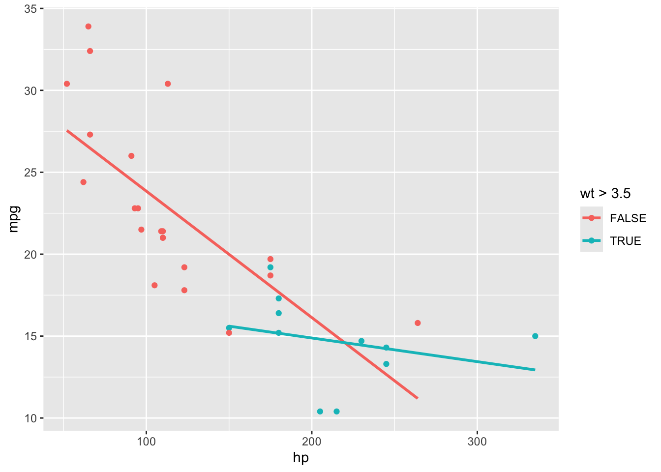
In a previous lecture, we saw how we could incorporate an interaction term between a quantitative and a categorical feature. This results in a “dummy” variable being either 0 or 1. We can also incorporate interaction terms using two quantitative features. We might look into interaction terms if we have reason to believe the relationship between the two predictor variables and the outcome variable is influenced by an interaction of the two predictors. To see this, we will look at the mtcars dataset. In the visualization below, we can see a change in the outcome (mpg), caused by an impact between two features (hp and wt), where the level of one feature is impacting how the other feature contributes to that outcome.
summary(lm(mpg ~ hp + wt, mtcars))
Call:
lm(formula = mpg ~ hp + wt, data = mtcars)

Residuals:
   Min     1Q Median     3Q    Max
-3.941 -1.600 -0.182  1.050  5.854

Coefficients:
            Estimate Std. Error t value Pr(>|t|)
(Intercept) 37.22727    1.59879  23.285  < 2e-16 ***
hp          -0.03177    0.00903  -3.519  0.00145 **
wt          -3.87783    0.63273  -6.129 1.12e-06 ***
---
Signif. codes:  0 '***' 0.001 '**' 0.01 '*' 0.05 '.' 0.1 ' ' 1

Residual standard error: 2.593 on 29 degrees of freedom
Multiple R-squared:  0.8268,    Adjusted R-squared:  0.8148
F-statistic: 69.21 on 2 and 29 DF,  p-value: 9.109e-12
The summary seen below shows the model with an interaction term present. This shows us that mpg is not just the sum of hp and wt, but rather the sum plus some interaction between the two variables.
summary(lm(mpg ~ hp*wt, mtcars)) # same as mpg ~ hp + wt + hp:wt
Call:
lm(formula = mpg ~ hp * wt, data = mtcars)

Residuals:
    Min      1Q  Median      3Q     Max
-3.0632 -1.6491 -0.7362  1.4211  4.5513

Coefficients:
            Estimate Std. Error t value Pr(>|t|)
(Intercept) 49.80842    3.60516  13.816 5.01e-14 ***
hp          -0.12010    0.02470  -4.863 4.04e-05 ***
wt          -8.21662    1.26971  -6.471 5.20e-07 ***
hp:wt        0.02785    0.00742   3.753 0.000811 ***
---
Signif. codes:  0 '***' 0.001 '**' 0.01 '*' 0.05 '.' 0.1 ' ' 1

Residual standard error: 2.153 on 28 degrees of freedom
Multiple R-squared:  0.8848,    Adjusted R-squared:  0.8724
F-statistic: 71.66 on 3 and 28 DF,  p-value: 2.981e-13
The equation for this model will be the following: \[\textbf{Model Equation: } \text{mpg} = 49.81 - 0.12\cdot\text{hp} - 8.22\cdot\text{wt} + 0.03\cdot\text{hp}\cdot\text{wt}\]
We can interpret the feature coefficients as the mean outcome change for 1 unit of change in the feature, holding all other features constant. When it comes to interpreting the interaction coefficient we will say the coefficient is the mean outcome change for a 1 unit change in feature conditioned on the other interaction feature. This result will depend on the value of the second variable.
We can see below that depending on what one value is for the interaction term will affect the slope/interpretation of the other interaction term: \[\begin{align*}
\textbf{For wt = 2.4:} \quad & 30.09 - 0.05\cdot \text{hp}\\
\textbf{For wt = 3.4:} \quad & 21.87 - 0.03\cdot \text{hp}\\
\textbf{For wt = 4.4:} \quad & 13.66 - 0.002\cdot \text{hp}
\end{align*}\]