attendance <- c(12, 13, 13, 14, 15, 15, 17, 17, 17, 18, 18, 19, 20, 20)
grade <- c(45, 60, 45, 65, 80, 60, 70, 75, 90, 85, 70, 90, 90, 100)
plot(attendance, grade, main="Scatter Plot: Attendance vs. Grade")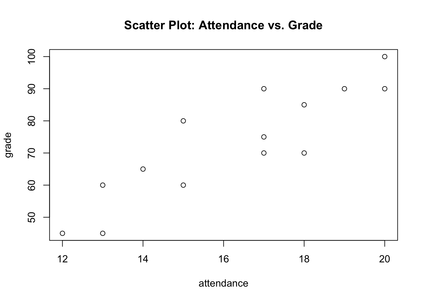
There are many different tools and potential applications within the field of machine learning (which I will probably refer to as “statistical learning”). The three main application areas we will discuss in this course are regression (predicting a quantitative value like the price of a house), classification (predicting a qualitative value like whether a tumor is benign or malignant), and clustering (grouping similar values together). We will go into more detail on all of these in due time, but I want to just jump straight into the field by looking at one of the first methods developed: Simple Linear Regression. This method was formulated independently in the early 1800’s by Legendre and Gauss to predict planetary movements.
Let’s look at an example to understand what Simple Linear Regression consists of. Below we have the attendance records and the final grades for 14 students who took Data 101. We might be interested in seeing whether students who attended more classes tended to earn higher grades or even seeing if we can predict a student’s grade if we know how many classes they attended. This can help us see whether attendance is associated with a student’s grade and whether attendance may be useful for predicting grade. To see this, we can visualize the data using a scatter plot in R:
attendance <- c(12, 13, 13, 14, 15, 15, 17, 17, 17, 18, 18, 19, 20, 20)
grade <- c(45, 60, 45, 65, 80, 60, 70, 75, 90, 85, 70, 90, 90, 100)
plot(attendance, grade, main="Scatter Plot: Attendance vs. Grade")
Notice that there appears to be a positive linear relationship between the two variables, meaning that as attendance increases the grade in the course also tends to increase. We will typically plot the independent variable (the cause, the predictor) on the x-axis and the dependent variable (the effect, the outcome) on the y-axis. In this example, attendance is the predictor variable because we are using it to help predict the final grade, while grade is the outcome variable because it is the value we are trying to explain or predict.
The basic idea of simple linear regression is coming up with a line of best fit that best describes the relationship between the two variables. Since we will be discussing a line, we should mention that it must have the form \(y=mx+b\) where \(b\) is the y-intercept, the point \((0,b)\), and \(m\) is the slope, often thought of as “rise over run”. For our case, \(x\) is the independent variable (the variable we think causes a change in another variable), and \(y\) is the dependent variable (the variable we want to explain).
We will discuss them in more detail later, but there are a few assumptions we will need to verify before carrying out simple linear regression. The first is that we have a linear relationship between \(x\) and \(y\) (…go figure). Secondly, we need to confirm that our observations are independent of each other, which means one observation is not influenced by any of the other observations. Finally, we will want to (visually) check that the variables exhibit homoscedasticity, which essentially means that the variance is equal across the visualization.
Going back to our example, there are a few different lines that we could draw as possible lines of best fit (though not all of them are good). For instance, we could just decide to draw a horizontal line which is the average of the grades, but it does not take into account the other variable (attendance). We could also play around with different slopes and intercepts and see if we get one that best represents the trend of the data. In the end, we will aim to choose a line that is close to all of the points simultaneously.
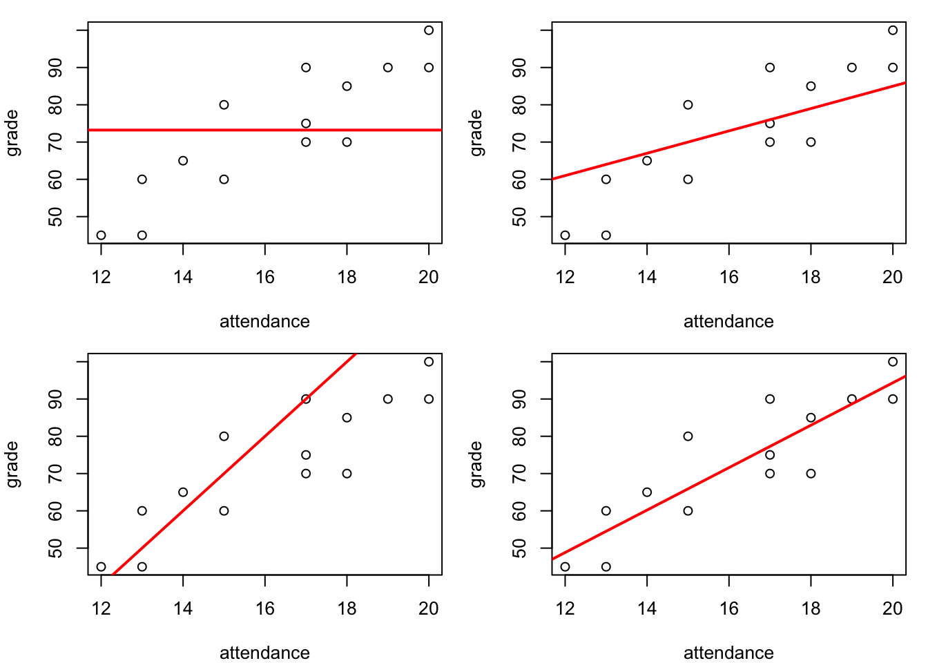
In the figure above, we can probably determine that the bottom right plot is the best among the four, but how do we know it is the best among all possible lines? To answer this question, we will need to introduce the idea of residuals. Residuals tell us how far off a predicted value is from the actual value. We could quantify it as: \[\text{Residual}=y-\hat{y}\]
where \(\hat{y}\) is our predicted value (the value on the line of best fit at the same \(x\) value). Just as a quick note, normally in statistics if a variable has a “bar” on top of it then it represents the mean (like \(\bar{y}=\) the mean of \(y\)) and if a variable has a “hat” on top of it then it represents a predicted value (like \(\hat{y}\)).
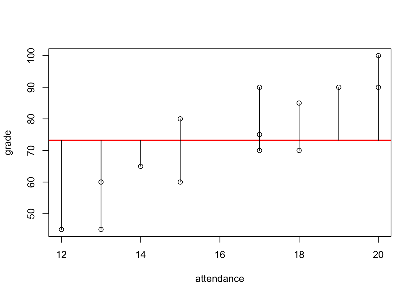
We can visualize this using our vertical line of best fit. The red line is our prediction (the line of best fit) and the vertical lines are our residuals (how far off our predicted value is from the actual value). When our actual value is less than our predicted value the residual will be negative, and it will be positive if the actual value is greater than the predicted value. We can then sum our residuals and show that the value is 0 for this instance (it is not exactly 0 due to rounding early on in the problem).
grade_bar = round(mean(grade), 2) # Rounding mean to 2 decimal place
grade_bar
[1] 73.21grade [1] 45 60 45 65 80 60 70 75 90 85 70 90 90 100grade_residual_horizontal <- grade - grade_bar
grade_residual_horizontal [1] -28.21 -13.21 -28.21 -8.21 6.79 -13.21 -3.21 1.79 16.79 11.79
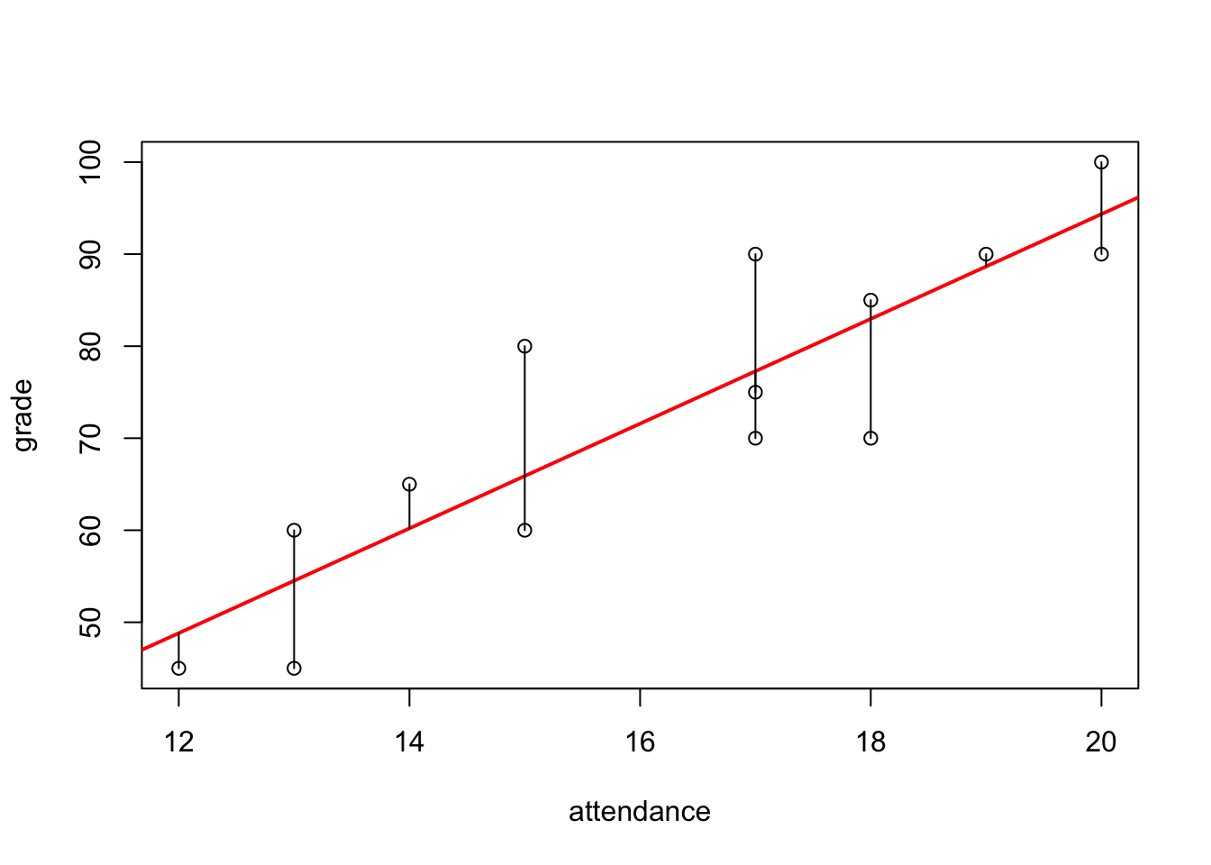
[11] -3.21 16.79 16.79 26.79sum(grade_residual_horizontal) # It is really 0 but we have a rounding error[1] 0.06Let’s also look at the plot with the residual lines for the regression model we thought was the best one. Notice that overall the residuals are smaller but the sum of the residuals is once again 0 like in the previous example.
grade_residual_optimal # residuals from optimal line of best fit 1 2 3 4 5 6 7 8 9 10 11
-3.82 5.49 -9.51 4.80 14.10 -5.90 -7.28 -2.28 12.72 2.03 -12.97
12 13 14
1.34 -4.36 5.64 sum(grade_residual_optimal) # It is really 0 but we have a rounding error[1] -3.552714e-15The optimal line of best fit will be the line closest to all of the points, thus minimizing the residuals. But, we have just seen two examples where the sum of the residuals is 0 but the lines are very different from each other. This is because any line that goes through the point \((\bar{x}, \bar{y})\) will have the residuals sum to 0 (much like how the deviations sum to 0 when we calculate the standard deviation). To get around this issue we will do something similar to calculating the standard deviations– we will square the errors, calculate the mean, and then take the square root. We will call this measurement the RMSE (Root Mean Square Error). Whenever you do it, just work through the acronym backward (find Error, Square them, calculate the Mean, take the square Root). Our simple linear regression line will be the line that results in the minimum RMSE.
# Calculating the RMSE for the Horizontal Line of Best Fit
grade_residual_horizontal
[1] -28.21 -13.21 -28.21 -8.21 6.79 -13.21 -3.21 1.79 16.79 11.79
[11] -3.21 16.79 16.79 26.79sqrt(mean(grade_residual_horizontal^2))[1] 16.43245# Calculating the RMSE for the Perceived Line of Best Fit
grade_residual_optimal 1 2 3 4 5 6 7 8 9 10 11
-3.82 5.49 -9.51 4.80 14.10 -5.90 -7.28 -2.28 12.72 2.03 -12.97
12 13 14
1.34 -4.36 5.64 sqrt(mean(grade_residual_optimal^2))[1] 7.731126Now that we know the simple linear regression line will be the line that minimizes the RMSE we might ask ourselves, how do we find the line which actually has the minimum RMSE value? To do so, we want to determine the coefficients \(a\) and \(b\) such that
\[\sum (y_i - \hat{y})^2 = \sum (y_i - (a + bx_i))^2 \]
is minimized. We do not want to try every possible combination of \(a\) and \(b\) (as there are infinitely many possibilities after all!). To figure this question out, we will need a little bit of calculus to optimize the function using partial derivatives. Since the actual derivation is not important for this class I will leave the proof as an exercise for the reader. If one were to work out the problem, one would find that the coefficients which minimize the RMSE are:
\[a = \bar{y} - b\bar{x} \qquad \text{and} \qquad b = \frac{\sum(x_i - \bar{x})(y_i - \bar{y})}{\sum(x_i - \bar{x})^2} = \frac{\text{cov}(x,y)}{\text{var}(x)}\]
Note that variance is \(\frac{1}{n-1} \sum (x_i - \bar{x})^2\) and covariance is \(\frac{1}{n-1} \sum(x_i - \bar{x})(y_i - \bar{y})\) thus allowing us to make the simplification. With this information, we can show that the coefficients for the simple linear regression model will be:
x <- attendance
y <- grade

b <- sum((x - mean(x))*(y-mean(y)))/sum((x-mean(x))^2)
b
[1] 5.691824cov(x,y)/var(x)[1] 5.691824a <- mean(y) - b*mean(x)
a[1] -19.48113Therefore, the simple linear regression model would be described by the line:
\[ \text{Grade} = 5.69 * \text{Attendance} - 19.48\]
plot(attendance, grade)
abline(a=a, b=b, col="red", lwd=2) # a is intercept and b is slope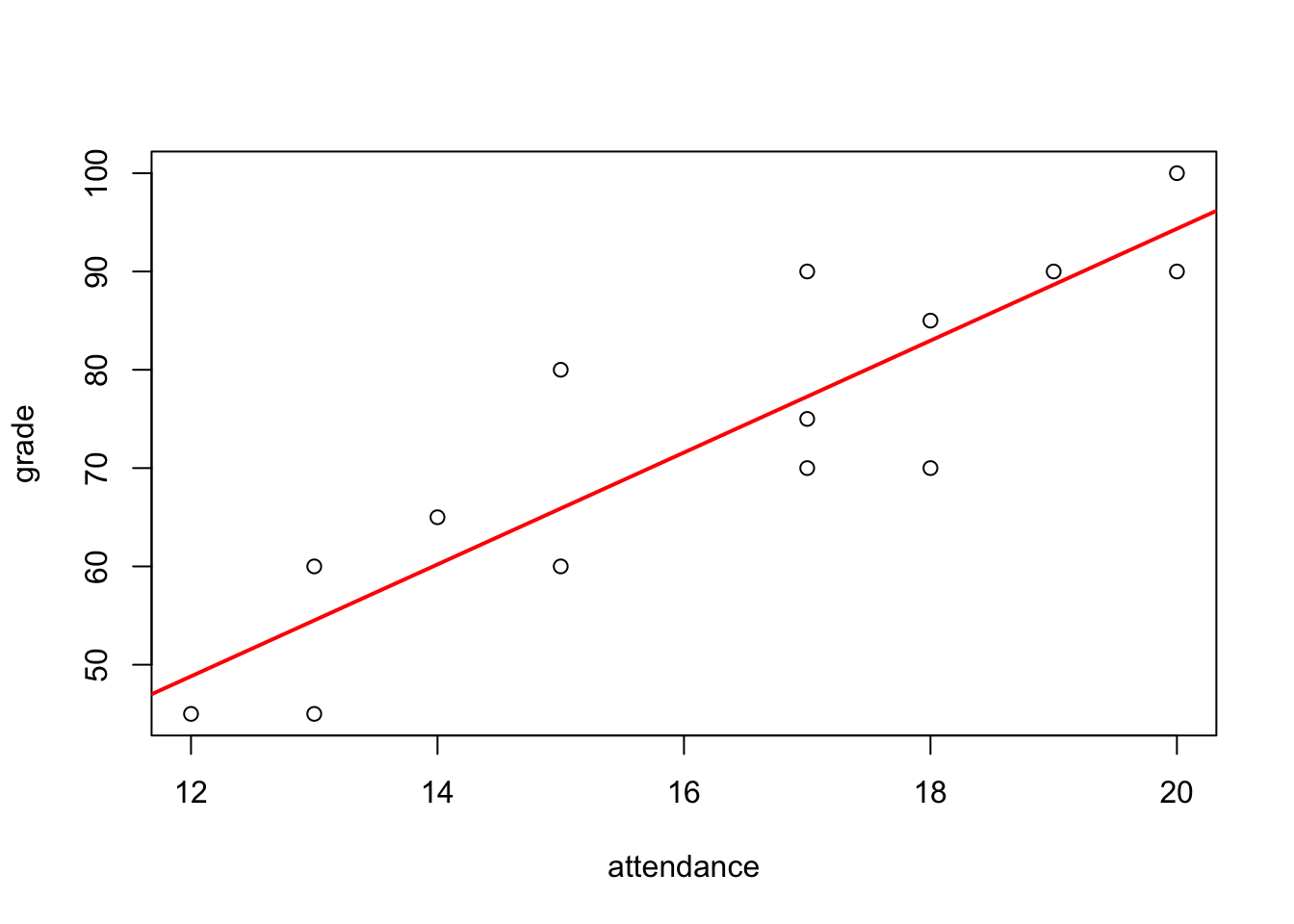
Luckily, we do not have to manually do these calculations, as there is a function in R that will allow us to create a linear model. To do so, we will use the lm() function. We will specify the dependent variable (outcome) then place a tilde (found under the escape key) and then specify the independent variable (predictor). In doing so, we can see that we end up with the same result as doing it “manually”.
lm(grade ~ attendance)
Call:
lm(formula = grade ~ attendance)

Coefficients:
(Intercept)   attendance
    -19.481        5.692
So, if we had a student who would only be able to attend 17 classes, we could predict their final grade in the class as follows:
\[\text{Grade} = 5.69 * (17) - 19.48 = 77.25\]
We saw previously that the Simple Linear Regression (SLR) model is the closest line to all of the points simultaneously, meaning that the Root Mean Square Error (RMSE) is minimized. The line of best fit will (usually) never cross through every point due to some “noise” in the data. To explain why our model is never perfect, we will introduce the idea of the error component epsilon (\(\epsilon\)). In doing so, we can formalize our simple linear regression model as follows:
\[y = \beta_0 + \beta_1 x + \epsilon\]
We will utilize \(\beta_0\) as the y-intercept and \(\beta_1\) as the slope. In order for us to use a simple linear model the error term, \(\epsilon\), should follow a normal distribution with a mean of 0 and a variance of \(\sigma^2\), meaning \(\epsilon \sim N(0, \sigma^2)\). This means that the errors should be centered around 0, so our model is not consistently overpredicting or underpredicting. It also means that most errors should be relatively small, while larger errors should be less common. This assumption becomes especially important when we use the model to create confidence intervals, conduct hypothesis tests, and interpret p-values.
So, we were able to determine that the line of best fit to be: \[\text{Grade} = 5.69 * \text{Attendance} - 19.48 + \epsilon\]
It is vital that we understand how to interpret the coefficients and output of this model. When looking at the intercept, we can say that when \(x=0\) the estimated \(\hat{y}\) will be \(\beta_0\). It will not always be plausible to interpret the intercept though, as sometimes it is not possible for it to occur. Interpreting the slope is a little different, it tells us that the estimated change in \(\hat{y}\) per unit increase of \(x\) is \(\beta_1\).
For our case, the intercept tells us that students who attend 0 classes will on average receive a grade of -19.48 (\(5.69*0 - 19.48\)). Likewise, the slope for attendance informs us that for every increase of 1 class attended, the predicted grade increases of 5.69, on average (\(5.69*10 - 19.48= 37.42\) and \(5.69*11 - 19.48=43.11\) giving an increase of \(5.69\)). We can then make predictions and substitute a value for the Attendance total:
As a general rule of thumb, we should avoid making predictions for values that are far outside the range of our observed data. This is called extrapolation. In our example, we only have data on students who attended between 12 and 20 classes, so we should be cautious about making predictions for attendance values outside of that range. For instance, we would not want to make a strong claim about the average grade for a student who attends only 4 classes. While we could plug 4 into the regression equation, we do not know whether the linear relationship between attendance and grade continues that far beyond the data we actually observed.
When we look at the model in R, we are only presented with the coefficient values. We will want more information than that, and luckily R gives us a lot of information relating to our model using the summary() function. This includes information on the residuals, the coefficients, the R-squared value, and the F-statistic; all of which we will discuss.
model <- lm(grade~attendance)
summary(model)
Call:
lm(formula = grade ~ attendance)

Residuals:
     Min       1Q   Median       3Q      Max
-12.9717  -5.5110  -0.4717   5.3145  14.1038

Coefficients:
            Estimate Std. Error t value Pr(>|t|)
(Intercept) -19.4811    14.4416  -1.349    0.202
attendance    5.6918     0.8761   6.497 2.95e-05 ***
---
Signif. codes:  0 '***' 0.001 '**' 0.01 '*' 0.05 '.' 0.1 ' ' 1

Residual standard error: 8.351 on 12 degrees of freedom
Multiple R-squared:  0.7786,    Adjusted R-squared:  0.7602
F-statistic: 42.21 on 1 and 12 DF,  p-value: 2.951e-05
One thing we mentioned earlier in this lecture was the fact that the error term (residuals) should be normally distributed centered around 0. We can look at a summary of the residuals in order to verify that this assumption may be true. If we recall from Data 200, we were able to do “Quartile-Analysis” on the data in order to determine if it is symmetric. We can see that the residuals are centered roughly around 0 and the distance between similar quartiles is roughly the same, causing no major concerns. We will have a more in-depth look at the residuals in a future lecture.
summary(model$residuals) Min. 1st Qu. Median Mean 3rd Qu. Max.
-12.9717 -5.5110 -0.4717 0.0000 5.3145 14.1038 Another thing worth taking a deeper look into is information regarding the coefficients. We have already seen how to calculate the estimates for the coefficients and how to interpret them.
summary(model)$coefficients Estimate Std. Error t value Pr(>|t|)
(Intercept) -19.481132 14.441601 -1.348959 0.202255
attendance 5.691824 0.876111 6.496693 0.000030While the estimate values are useful, they do not tell us the full story of what is happening with the model. For instance, maybe the coefficients are not statistically significant, and the way we will be able to make that determination is by looking at the Standard Error. We will not need to derive it in this course or have it memorized, but the formulas for the standard error (which helps measure the uncertainty of the estimate) can be found as:
\[ \text{se}\_b = \sqrt{\frac{\sum (y_i - \hat{y})^2}{n-2} / \sum(x_i - \bar{x})^2} \qquad \text{ and } \qquad \text{se}\_a = \sqrt{\frac{\text{se}^2_b*\sum x_i^2}{n}}\]
where \(\text{se}_b\) is the standard error for the slope coefficient, and \(\text{se}_a\) is the standard error for the intercept coefficient.
x <- attendance
y <- grade
y_hat <- 5.691824*x - 19.481132
n <- length(x)
se_b <- sqrt( (sum((y-y_hat)^2)/(n-2)) / sum((x-mean(x))^2) )
se_b
[1] 0.876111se_a <- sqrt(se_b^2 *sum(x^2)/(n))
se_a[1] 14.4416Calculating these standard errors is important for us as it will allow us to see if a calculated estimate is “unusual”. To determine if a coefficient is statistically significant (or “unusual”) we will need to perform a hypothesis test. Our initial assumption is that the intercept and slope coefficient are both 0. Thus, our two hypothesis tests will be formulated to see if the value is different than 0. Below we can see the null and alternative hypotheses as well as the formula for the test statistic:
\[ H_0 : \beta_0 = 0 \qquad \text{ and } \qquad H_1: \beta_0 \neq 0 \qquad \text{ with } \qquad T = \frac{\beta_0 - 0}{\text{se}_a} \]
as well as
\[ H_0 : \beta_1 = 0 \qquad \text{ and } \qquad H_1: \beta_1 \neq 0 \qquad \text{ with } \qquad T = \frac{\beta_1 - 0}{\text{se}_b}\]
So, after we calculate the test statistic, we can then use the Student’s t-distribution to calculate the p-value. When using the student’s t-distribution, your degrees of freedom in this instance will be \(df=n-2\) since 2 values are known (the intercept and the slope coefficient). Once this is completed, we can then compare the p-value to the level of significance (usually 0.05) to determine if the coefficient is statistically significant. As a reminder, the p-value tells us the probability of observing the test statistic or a more extreme value assuming the null hypothesis is true. A low p-value would then indicate that the probability of obtaining the test statistic by chance is small and thus we would reject the null hypothesis and conclude the coefficient is statistically different than 0. The summary output in R will help us see which estimates are significant based on the number of asterisks beside them (the more asterisks the smaller the p-value).
t_a <- -19.4811/se_a
t_a
[1] -1.348957pt(t_a, df=n-2)*2[1] 0.2022558t_b <- 5.6918/se_b
t_b[1] 6.496666(1-pt(t_b, df=n-2))*2[1] 2.950896e-05With this information completed, we can state that for our example the intercept estimate is not statistically different than 0 and the slope estimate is statistically different than 0.
Another piece of information we can gain from the summary is the F-statistic and the p-value associated with it. The F-statistic is usually used to test variance, and for this case, the F-test checks whether the model as a whole is useful. In simple linear regression, this is equivalent to testing whether the slope coefficient is different from 0. In multiple regression, it tests whether at least one predictor has a nonzero slope. We will not bother ourselves with the formula for this test statistic, but we should be aware that the hypothesis relating to this is:
\[ H_0: \text{ all slope coefficients are 0 } \qquad \text{ and } \qquad H_1: \text{ some coefficients are not 0} \]
If the p-value associated with this test statistic is significant it does not imply that all slope coefficients differ from 0, rather it indicates that at least one differs from 0. For our case, we can see the p-value associated with the overall model is extremely small, resulting in at least one coefficient differing from 0. This should be checked before we look at the coefficients, and if this is significant then we will look at the significance of the coefficients.
model <- lm(y~x)
x <- attendance
y <- grade
n <- length(x)

model <- lm(y~x)
sum((model$fitted.values - mean(y))^2) /
    (sum((y - model$fitted.values)^2)/(n-2))
[1] 42.207021-pf(42.20702, df1=1, df2=n-2)[1] 2.950777e-05The last thing we will discuss is the R-squared (\(R^2\)) value which is presented in the summary output of the model. This is called the coefficient of determination and measures the variability in the data that is explained in the model. Ideally, we want a model with an \(R^2\) value closer to 1, as that indicates the model does a good job of explaining the variance of the data. The calculation for \(R^2\) is done using the Residual Sum of Squares (RSS) which allows us to see the variability of our predictions, and the Total Sum of Squares (TSS) which allows us to see the variability of the data.
\[ \text{RSS } = \sum(y_i - \hat{y})^2 \quad \text{and} \quad \text{TSS } = \sum(y_i - \bar{y})^2 \quad \text{giving us} \quad R^2 = \frac{\text{TSS - RSS}}{\text{TSS}} = 1 - \frac{\text{RSS}}{\text{TSS}} \]
1-(sum((model$fitted.values - grade)^2) / sum((grade - mean(grade))^2))[1] 0.7786265summary(model)$r.squared[1] 0.7786265cor(attendance, grade)^2[1] 0.7786265It should be mentioned that \(R^2\) (the coefficient of determination) is different than \(r^2\) (the correlation squared). When dealing with regression based on Ordinary Least Squares (OLS) the values will be the same, but in general and later on in the course, the values will be different. We can interpret the results though as our model explains 77.86% of the variability of the data (since \(R^2=0.7786\)).