While there are many advantages for decision trees (such as interpretability), they do suffer from not being the most accurate compared to other models. Additionally, decision trees tend to have high variance, meaning that when we build a tree with different training data we will potentially end up with vastly different trees. This fact can be seen below if we build 2 trees using different splits of the training data. One split has 6 terminal nodes while the other has 11 terminal nodes, indicating that the trees have high variance since changes in the training data lead to large changes in the model. For this example, we are using the Boston dataset in the MASS library and trying to predict the median home price.
Regression tree:
tree(formula = medv ~ ., data = Boston, subset = train)
Variables actually used in tree construction:
[1] "rm"    "lstat" "nox"
Number of terminal nodes:  6
Residual mean deviance:  16.64 = 4110 / 247
Distribution of residuals:
    Min.  1st Qu.   Median     Mean  3rd Qu.     Max.
-23.0600  -2.4500  -0.1322   0.0000   1.9680  23.5700
Regression tree:
tree(formula = medv ~ ., data = Boston, subset = train)
Variables actually used in tree construction:
[1] "rm"    "lstat" "dis"   "nox"
Number of terminal nodes:  11
Residual mean deviance:  12.05 = 2916 / 242
Distribution of residuals:
    Min.  1st Qu.   Median     Mean  3rd Qu.     Max.
-14.5700  -1.6710  -0.1037   0.0000   1.6370  18.2800
Let’s also take a look at how our model does on the testing dataset by calculating the RMSE so we can compare it with different models that we build.
test <- Boston[-train,]pred <-predict(Boston_tree, newdata=test)sqrt(mean((pred - test$medv)^2))
[1] 5.008067
To combat these issues, we can introduce the idea of an ensemble method, which combines multiple simple models into a single (potentially) more powerful model. The three that we will focus on when dealing with decision trees are bagging, random forests, and boosting.
13.2 Bagging
The basic idea of bagging is to build a whole bunch of decision trees using different subsets of the training data and then when one wants to make a prediction they calculate the outcome for each decision tree and then average the results to determine the final outcome. Obtaining different subsets of the training data is accomplished with bootstrapping (a fancy word for sampling with replacement) which allows us to get many samples of the same size but with different combinations of training data. After this is done the trees are built and the outcomes are averages for regression. This method is useful because it reduces variance and it avoids overfitting but it does not necessarily reduce bias.
library(randomForest)
randomForest 4.7-1.2
Type rfNews() to see new features/changes/bug fixes.
Call:
 randomForest(formula = medv ~ ., data = train, mtry = 13, importance = TRUE)
               Type of random forest: regression
                     Number of trees: 500
No. of variables tried at each split: 13

          Mean of squared residuals: 14.11248
                    % Var explained: 81.53
pred <-predict(Boston_bag, newdata=test)sqrt(mean((pred - test$medv)^2))
[1] 3.825933
When looking at the results from above, we can see that 500 different decision trees were built with different combinations/sets of training data formed with bootstrapping (done behind the scenes). We define the argument mtry=13 because there are 12 predictor variables in our model that we want to look at for each decision split. When evaluating this model on the test data, we can notice the test RMSE is roughly 3.73, which is a decrease from the single decision tree test RMSE of 5.
13.3 Random Forests
Random Forests will employ a similar technique in that it too will build multiple models using bootstrapping from the training data. The main difference though is that random forests will only consider a random subset of predictors for each split within the tree. Typically at each split we only let the decision tree choose from \(\sqrt{p}\) predictors. This will ensure that each tree makes different decisions thus creating a diverse number of trees. Then since multiple diverse trees have been built (multiple trees make up a forest…make sense?!?) an average of the outcome values will be calculated to determine the predicted value. Random forests do enjoy the benefit of lower variance along with avoiding overfitting while also having better accuracy than a single decision tree.
Call:
 randomForest(formula = medv ~ ., data = train, mtry = sqrt(13),      importance = TRUE)
               Type of random forest: regression
                     Number of trees: 500
No. of variables tried at each split: 4

          Mean of squared residuals: 14.62974
                    % Var explained: 80.86
pred <-predict(Boston_rf, newdata=test)sqrt(mean((pred - test$medv)^2))
[1] 3.707396
It appears that the Random Forest model performed better than bagging due to the decrease in test RMSE to 3.56. When we built the model we specified the number of predictors it can look at for each split is only 4. This will lead to diverse trees which will help reduce the variance of the model and result in better predictive power.
13.4 Variable Importance
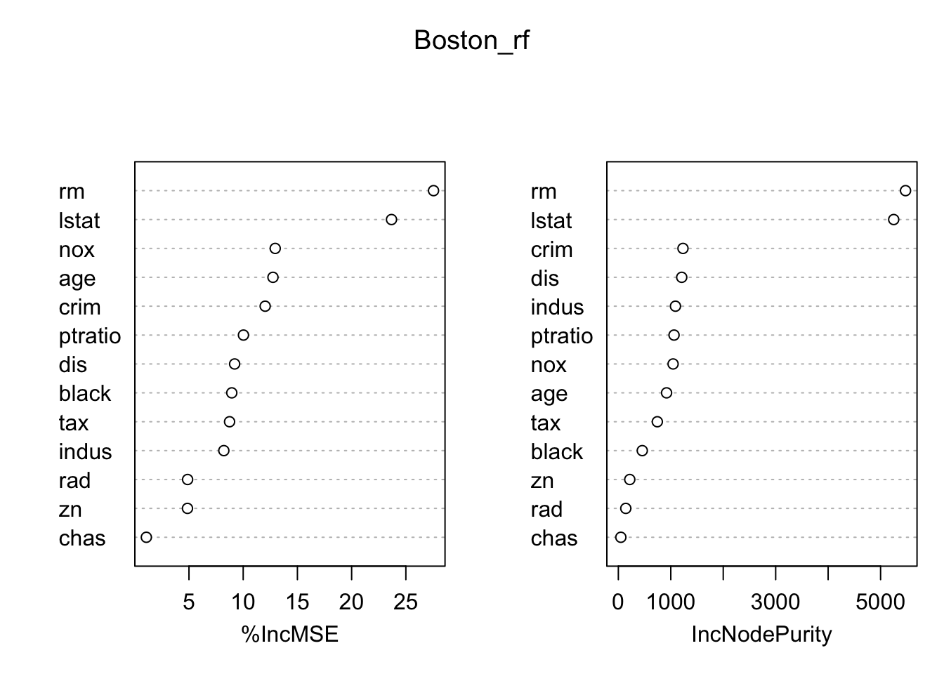
We can look at a plot of the predictor variables and see which ones are the most important to the model.
Looking at the output above, we could determine that the most important predictor variables in creating our decision trees and reducing the RSS within nodes are rm (number of bedrooms in the house) and lstst (percent of poverty in the area). Likewise, we can see that chas (if the house is on the river), zn (proportion of plots over 25,000 square feet), and rad (how close it is to the highway) are not very beneficial to the models for predicting the median home price.
13.5 Boosting
The last ensemble model that we will discuss relating to decision trees is boosting. This method starts with a simple decision tree and makes a prediction using the model. It then looks at which observations with the largest residuals and gives those observations more weight when it builds the next decision tree to try and correct the mistakes of the previous one. Boosting will slowly learn from the residuals by giving more weight to observations it routinely predicts wrongs. You may have encountered a similar algorithm if you have looked into gradient boosting. Once the model has been fully trained and all of the trees the outcome is then averaged using a weighted mean approach, with each model’s contribution weighted to its performance. This method produces higher accuracy but can potentially lead to overfitting of the data.
To create a boosting decision tree model in R, we will need the gbm() function in the gbm library. Additionally, if we are doing regression then we will need to specify the argument distribution = "gaussian" and if we are performing classification then the distribution would be “binomial”. We can also constrict the depth of each tree using the interaction.depth argument. Finally, you could play around with the shrinkage parameter (\(\lambda\)) to adjust the learning rate. You may have to play around with the argument parameters to hyper-tune the model.
gbm(formula = medv ~ ., distribution = "gaussian", data = train,
    n.trees = 5000, interaction.depth = 4, shrinkage = 0.05)
A gradient boosted model with gaussian loss function.
5000 iterations were performed.
There were 13 predictors of which 12 had non-zero influence.
pred <-predict(Boston_boost, newdata=test)
Using 5000 trees...
sqrt(mean((pred - test$medv)^2))
[1] 3.462711
Looking at the boosted model above, we can see that the test RMSE is roughly 3.4, a marked improvement on the standard decision tree test RMSE of 5. Choosing a different shrinkage value will result in a different learning rate while choosing a different (larger) number of trees may result in overfitting of the model.
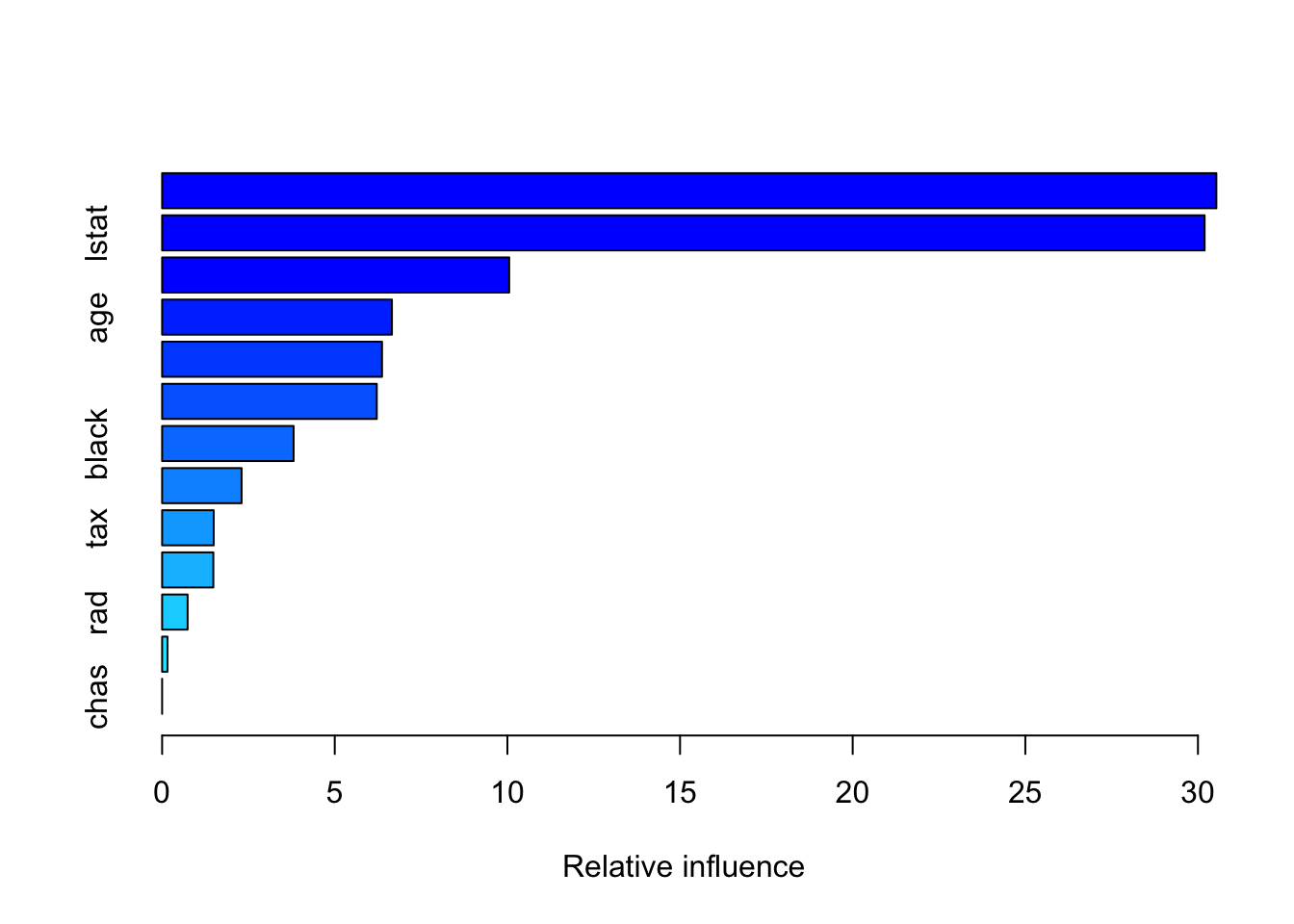
summary(Boston_boost)
            var    rel.inf
rm           rm 30.5330972
lstat     lstat 30.1929940
dis         dis 10.0530197
age         age  6.6557099
crim       crim  6.3687499
nox         nox  6.2169626
black     black  3.8078074
ptratio ptratio  2.3013597
tax         tax  1.4936203
indus     indus  1.4835627
rad         rad  0.7383420
zn           zn  0.1547746
chas       chas  0.0000000