So far in this course, we have spent a lot of time thinking about which variables should be included in a model and how those variables can be used to explain patterns in our data. In some situations, though, we may have too many variables describing very similar things. If several variables are strongly correlated with each other, we may be carrying around a lot of repeated information.
For example, suppose we are studying students and collect their scores on algebra, calculus, statistics, physics, chemistry, and several other quantitative courses. A student who performs well in one of these classes may also tend to perform well in many of the others. We could keep every individual variable, but perhaps much of the information could be summarized by a smaller number of underlying measurements such as “general quantitative performance.”
This is the basic idea behind Principal Component Analysis, usually abbreviated as PCA. PCA is an unsupervised learning method that takes a collection of quantitative variables and creates a smaller collection of new variables called principal components. These new variables are linear combinations of our original variables and are designed to capture as much of the variation in the original dataset as possible.
In the previous lecture on K-Means Clustering, our goal was to reduce the number of observations into a few meaningful groups. PCA tackles a different problem: we are trying to reduce the number of features needed to describe those observations.
16.1 Why Do We Need Dimensionality Reduction?
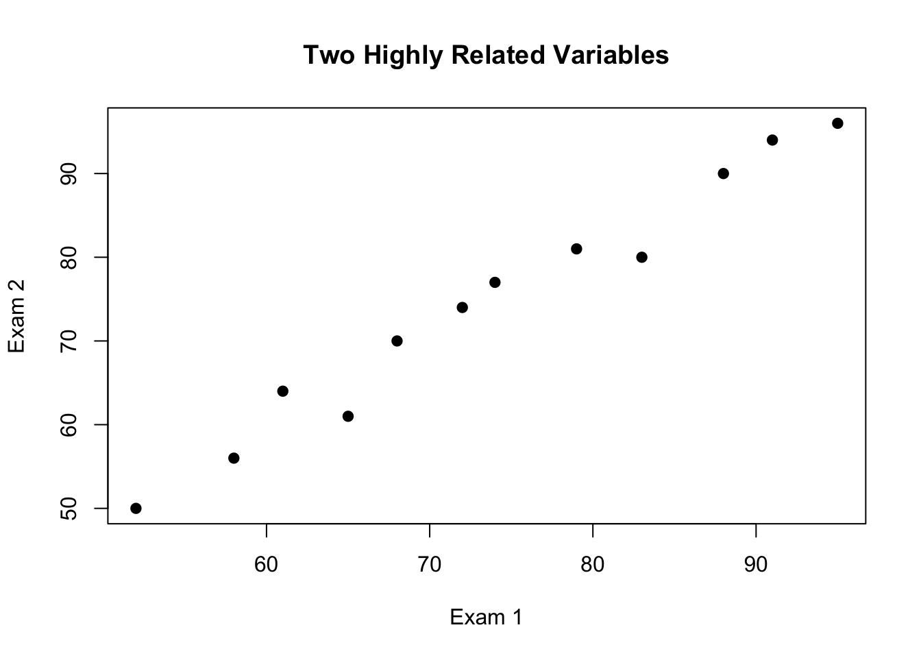
Let us begin with a small example. Suppose we collected two exam scores from a group of students:
We can also calculate the correlation between the two variables:
cor(exam_data$exam1, exam_data$exam2)
[1] 0.9868283
The two exams contain different information, but they are clearly related. Students with high Exam 1 scores also tend to have high Exam 2 scores. This means that keeping both variables may be somewhat redundant. Instead of keeping the two original measurements, imagine drawing a line through the data in the direction where the observations vary the most. We could then describe each student by how far they are located along that line. A student toward one end of the line would generally have lower scores, while a student toward the other end would generally have higher scores.
That new direction is essentially what the first principal component is trying to find. This becomes much more useful when we have a larger number of variables. Suppose we have 20 variables but many of them are strongly correlated. PCA may reveal that most of the information in those 20 variables can be represented reasonably well using only 3 or 4 new variables. Instead of working in 20 dimensions, we may be able to work in a much smaller space.
This process is called dimensionality reduction. There are several reasons we may want to reduce the dimensionality of a dataset:
We may be able to summarize a large number of related variables with only a few components.
We can visualize high-dimensional data using two or three principal components.
We can remove some redundant information caused by highly correlated features.
The principal components can sometimes be used as inputs for later machine learning models.
A smaller set of features may make patterns within the data easier to see.
Of course, reducing the number of variables comes with a cost. If we replace 20 variables with only 3 principal components, we will almost certainly lose some information. PCA is therefore trying to find a compromise: use fewer dimensions while retaining as much information as possible.
16.2 How Principal Components Are Created
To understand PCA, let us return to our two-exam example. We will standardize the two variables and then calculate the principal components using the prcomp() function.
Standard deviations (1, .., p=2):
[1] 1.4095490 0.1147682

Rotation (n x k) = (2 x 2):
            PC1        PC2
exam1 0.7071068 -0.7071068
exam2 0.7071068  0.7071068
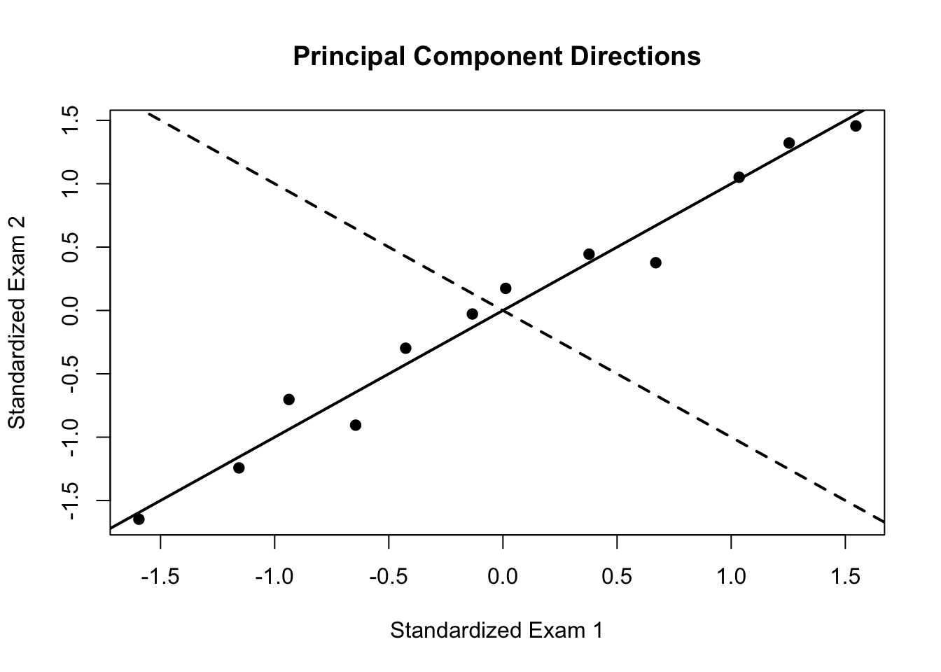
The first principal component, which we will call PC1, points in the direction where the data vary the most. The second principal component, PC2, must be perpendicular to PC1 and captures the largest remaining amount of variation.
PC1 follows the direction where the observations are spread out the most. PC2 is perpendicular to PC1 and describes the remaining variation that PC1 did not capture. In this example, PC1 will largely represent a student’s overall exam performance because both Exam 1 and Exam 2 increase together. PC2 will instead represent differences between the two exams. A student with a relatively high Exam 1 score but a relatively low Exam 2 score would move in one direction along PC2, while the opposite type of student would move in the other direction.
The important idea is that PCA does not simply select one of our existing variables. Instead, it creates entirely new variables by combining the original features.
For standardized variables \(z_1,z_2,\ldots,z_p\), the first principal component has the general form
\[PC_1=a_{11}z_1+a_{12}z_2+\cdots+a_{1p}z_p,\]
where the \(a\) values are weights describing how much each original variable contributes to the component. These weights are called loadings.
The second principal component will have a different set of weights:
\[PC_2=a_{21}z_1+a_{22}z_2+\cdots+a_{2p}z_p.\]
We can see the loadings for our exam example using:
Suppose PC1 gives similar positive weights to Exam 1 and Exam 2. Then a student with high standardized values on both exams will have a high PC1 score. This is why we might interpret PC1 as something like “overall exam performance.”
We can calculate the actual principal component scores for every student:
Loadings tell us how the original variables are combined to create a principal component.
Scores tell us where each observation falls on those principal components.
We can verify the basic calculation for the first student. Since we standardized the variables before performing PCA, we multiply the standardized Exam 1 and Exam 2 values by their PC1 loadings:
exam_scaled[1,]
    exam1     exam2
-1.594803 -1.647221
exam_pca$rotation[,1]
    exam1     exam2
0.7071068 0.7071068
sum(exam_scaled[1,] * exam_pca$rotation[,1])
[1] -2.292457
exam_pca$x[1,1]
      PC1
-2.292457
The two values should match apart from very small rounding differences. So, although PCA may initially sound complicated, each PC score is really just a weighted combination of the original variables.
PCA chooses the loadings so that PC1 captures the largest possible amount of variation in the data. PC2 then captures as much of the remaining variation as possible while being perpendicular to PC1. PC3 does the same thing after accounting for PC1 and PC2, and the process continues.
Because the principal components are perpendicular to one another, they are also uncorrelated:
This is one of the reasons PCA can be useful when the original variables are highly correlated. We replace a set of correlated features with a new set of uncorrelated components.
There is a more mathematical explanation involving eigenvalues and eigenvectors of a covariance or correlation matrix, but we do not need to derive those calculations in this course. The important thing for us is understanding what PCA is optimizing and how we can interpret the output.
16.3 Running PCA in R
Let us move to a dataset with more than two variables. We will once again use the iris dataset, which contains four quantitative measurements for 150 flowers.
Notice that several of the measurements are related to one another. In particular, Petal Length and Petal Width are very strongly correlated. This suggests that there may be some redundant information in the original four variables.
The rotation object contains the loadings, the x object contains the principal component scores for each flower, and sdev gives the standard deviation of each principal component.
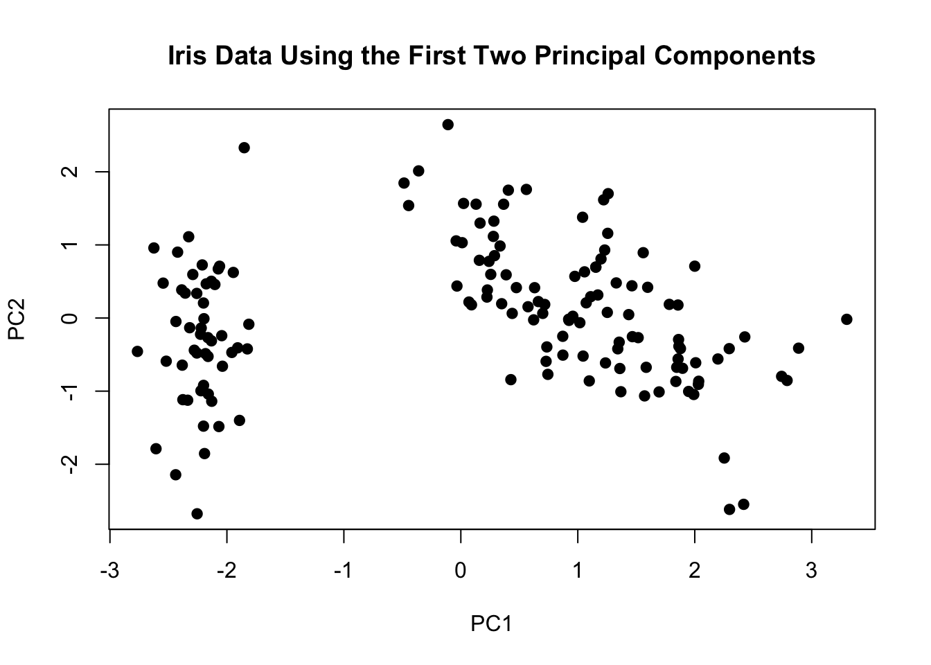
Since the first two principal components are now just two quantitative variables, we can plot all 150 flowers in two dimensions:
plot(iris_pca$x[,1], iris_pca$x[,2], pch=19,xlab="PC1", ylab="PC2",main="Iris Data Using the First Two Principal Components")
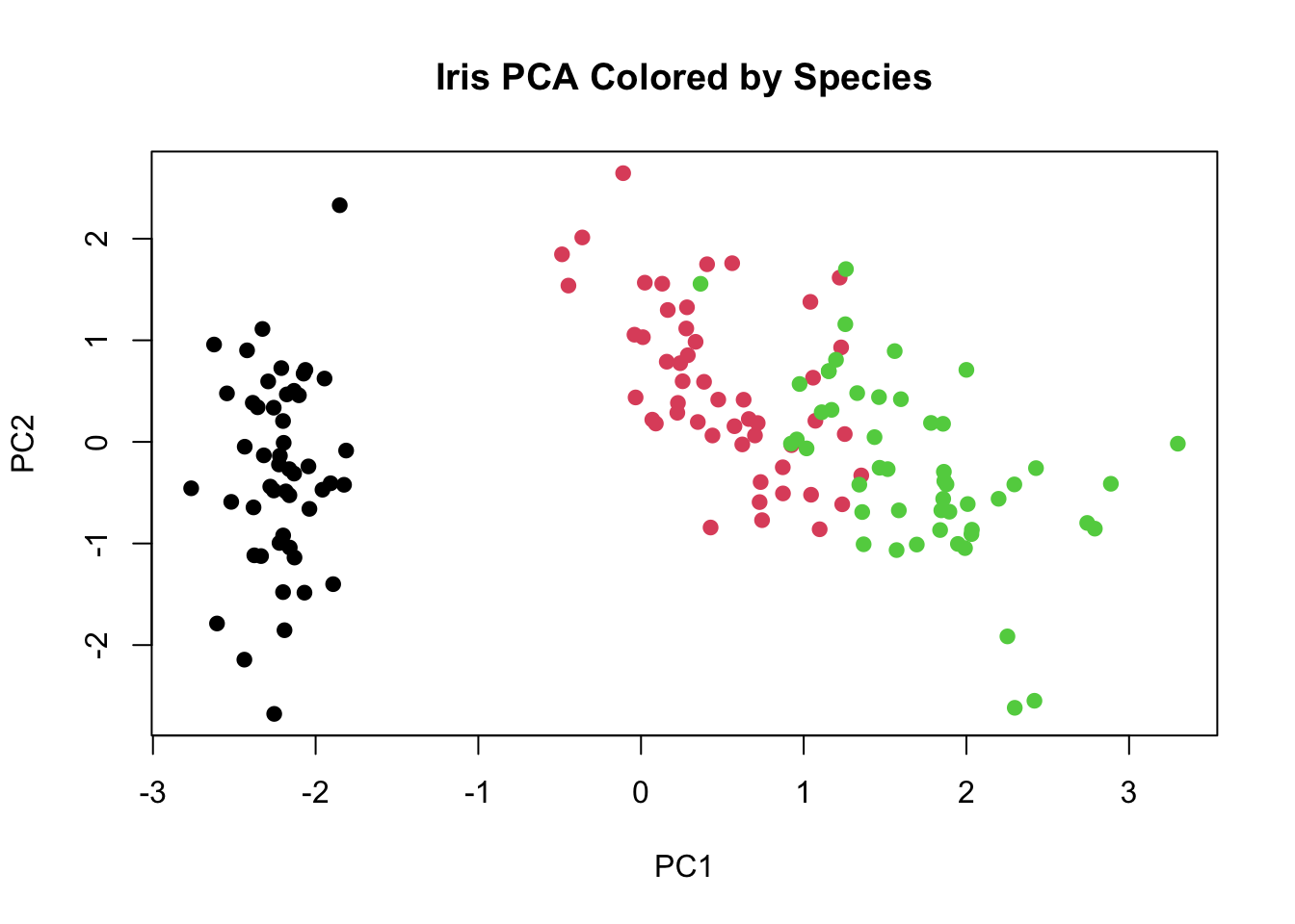
At this point, PCA has not used the flower species at all. It is still an unsupervised learning method. However, because we happen to know the species in this dataset, we can color the points afterward to see whether the PCA representation reveals any natural structure.
plot(iris_pca$x[,1], iris_pca$x[,2], col=as.numeric(iris$Species), pch=19,xlab="PC1", ylab="PC2", main="Iris PCA Colored by Species")
This is one of the major uses of PCA. It is impossible to directly make a scatter plot containing four axes, but PCA allows us to compress those four measurements into two new variables and visualize the observations in two dimensions.
We should be careful with our interpretation though. PC1 is not one single original feature and PC2 is not another. Each principal component contains information from all of the original variables.
We can inspect the loadings to determine which variables contribute the most:
For each component, variables with loadings farther from 0 contribute more strongly to that component. Variables with loadings closer to 0 have relatively little influence.
The sign also matters when comparing variables within the same component. If two variables have loadings with the same sign, larger values of those variables push observations in the same direction along that component. If they have opposite signs, they push observations in opposite directions.
However, the overall sign of a principal component is arbitrary. R could multiply every loading and every score for PC1 by \(-1\) and it would still represent exactly the same principal component. Therefore, we should not become too attached to whether a component points “left” or “right” in a plot. What matters is the relative pattern among the loadings.
we might find it easier to mentally reverse every sign and describe the same component as increasing with Sepal Length, Petal Length, and Petal Width while decreasing with Sepal Width. The statistical information has not changed.
16.4 How Much Information Does Each Component Explain?
So far we have created four principal components from the four variables in iris. If we keep all four components, we have not actually reduced the dimensionality of the data. We have simply rewritten the same information using a different coordinate system. The real benefit occurs when the first few principal components explain most of the variation in the original dataset. We can calculate the variance of each principal component by squaring the standard deviation:
pc_variance <- iris_pca$sdev^2pc_variance
[1] 2.91849782 0.91403047 0.14675688 0.02071484
We can then divide each variance by the total variance to determine the proportion of variance explained by each component:
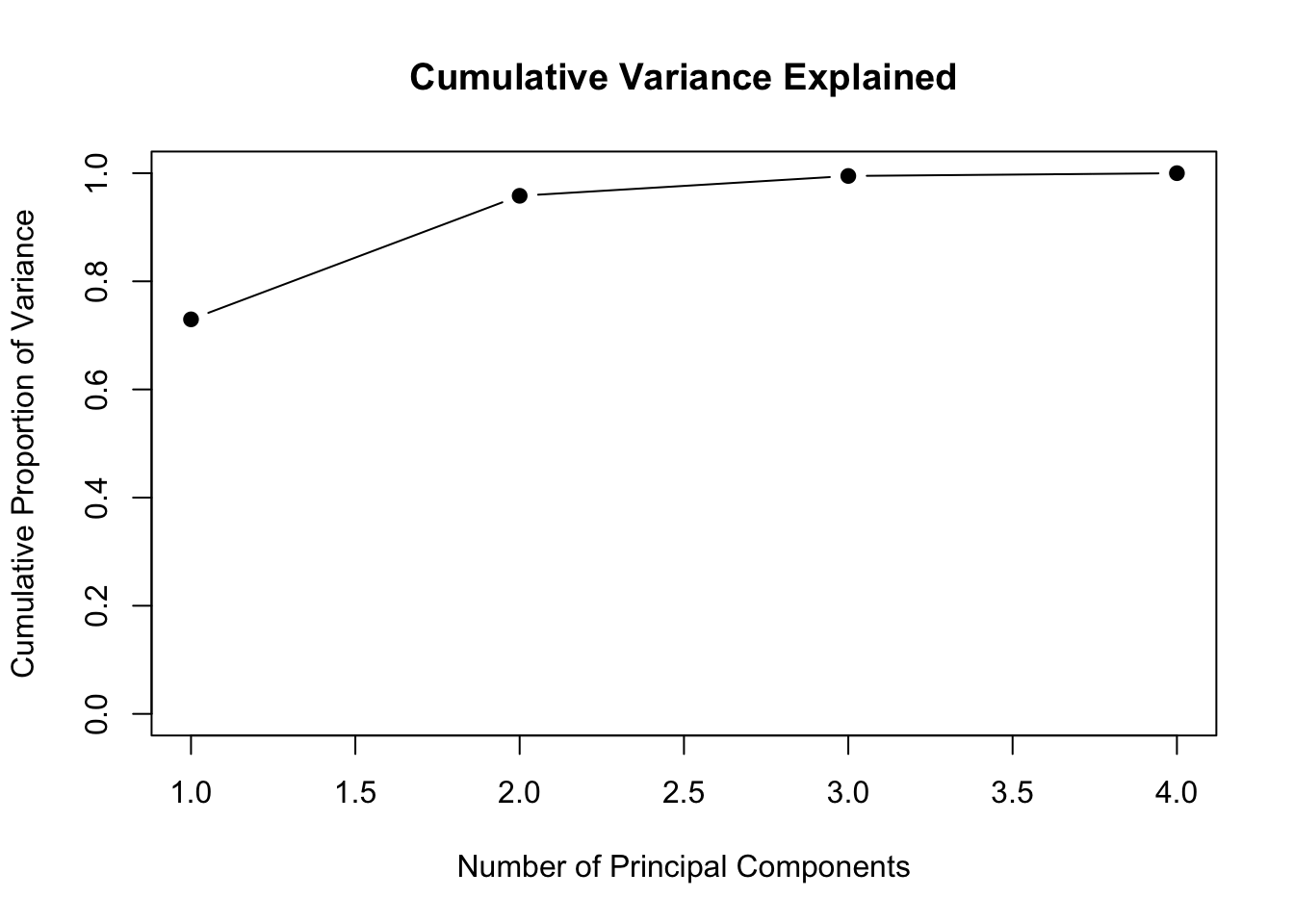
The cumulative proportion tells us how much information we retain if we keep the first 1, 2, 3, and so on principal components:
cumsum(prop_variance)
[1] 0.7296245 0.9581321 0.9948213 1.0000000
R will calculate this information for us automatically using:
summary(iris_pca)
Importance of components:
                          PC1    PC2     PC3     PC4
Standard deviation     1.7084 0.9560 0.38309 0.14393
Proportion of Variance 0.7296 0.2285 0.03669 0.00518
Cumulative Proportion  0.7296 0.9581 0.99482 1.00000
The Proportion of Variance row tells us how much variation each individual component explains, while the Cumulative Proportion row tells us how much is explained by all components up to that point.
For example, if PC1 explains 73% of the variation and PC2 explains another 23%, then using only the first two principal components would retain approximately 96% of the total variation while reducing four original variables down to two.
That is a pretty good trade: we have cut the number of dimensions in half while retaining most of the information in the original data.
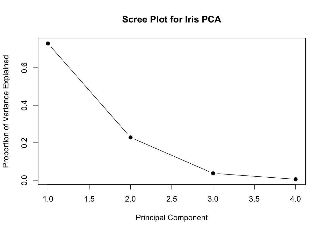
We can visualize this using a scree plot:
plot(prop_variance, type="b", pch=19,xlab="Principal Component", ylab="Proportion of Variance Explained",main="Scree Plot for Iris PCA")
We could also plot the cumulative proportion of variance:
plot(cumsum(prop_variance), type="b", pch=19, ylim=c(0,1),xlab="Number of Principal Components",ylab="Cumulative Proportion of Variance",main="Cumulative Variance Explained")
There is no universal rule saying that we must retain exactly 80%, 90%, or 95% of the variance. Those cutoffs can be useful guidelines, but the appropriate number of components depends on the goal of the analysis.
Much like choosing \(K\) in K-Means, we are balancing simplicity against information. Keeping more principal components preserves more of the original data, but it also reduces the benefit of dimensionality reduction.
16.5 Scaling and Interpreting the Components
Much like KNN and K-Means, PCA can be heavily affected by the scale of the variables. This is because PCA looks for directions with the largest amount of variance. A variable measured on a very large numerical scale will usually have a larger variance and can dominate the first principal components.
The variables are clearly measured on different scales. Assault has much larger values and a much larger standard deviation than the other variables. If we run PCA without scaling:
Importance of components:
                          PC1    PC2     PC3     PC4
Standard deviation     1.5749 0.9949 0.59713 0.41645
Proportion of Variance 0.6201 0.2474 0.08914 0.04336
Cumulative Proportion  0.6201 0.8675 0.95664 1.00000
Setting scale.=TRUE essentially tells R to place the variables on comparable scales before finding the principal components. In practice, this means PCA is working with standardized variables rather than the original measurements.
As a general rule, if the variables use substantially different units or numerical scales, scaling is usually a good place to start. If the variables are already measured on the same meaningful scale and differences in variance are important to the problem, we may choose not to scale.
16.6 PCA as Part of a Machine Learning Workflow
PCA can also be used as a preprocessing step before another machine learning method. Suppose we have a dataset containing many strongly correlated features. Rather than passing all of the original features into a model, we could first use PCA to create a smaller number of uncorrelated components and then fit the model using those components.
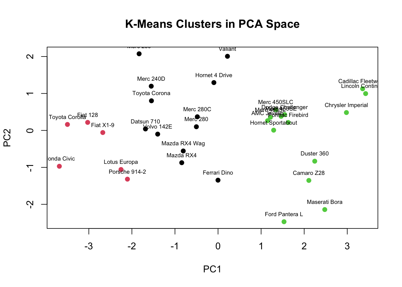
Let us connect this idea back to K-Means using mtcars. We will use six quantitative variables that describe the cars:
Several of these variables are strongly correlated. For example, heavier cars often have larger displacement and lower fuel efficiency. Rather than clustering on all six original variables, one option is to first perform PCA:
This combination is fairly common. PCA reduces the dimensionality of the dataset, and then a clustering method tries to identify groups in the reduced space.
However, we should not automatically assume that PCA will always improve a later model. PCA is designed to preserve variation, not necessarily the specific information that another model needs. A lower-variance component could still contain something important for prediction or clustering.
There is also an important warning if we use PCA as part of a supervised learning problem. Suppose we split data into a training set and testing set before fitting a classification or regression model. We should fit PCA using only the training data. Otherwise, information from the testing set would influence the transformation and we would introduce data leakage.
Conceptually, the process would be:
# Fit PCA using the training predictorspca_train <-prcomp(train_x, center=TRUE, scale.=TRUE)# Transform the training datatrain_pc <- pca_train$x[,1:k]# Apply the SAME transformation to the testing datatest_pc <-predict(pca_train, newdata=test_x)[,1:k]
The exact value of k would represent however many principal components we decided to retain.
This is the same general principle we have followed throughout machine learning: anything that learns information from the data should be learned using the training set and then applied to the testing set. PCA also has several limitations that we should keep in mind. One is that the principal components can be difficult to interpret, meaning the components combine all of the original variables rather than having one obvious meaning.