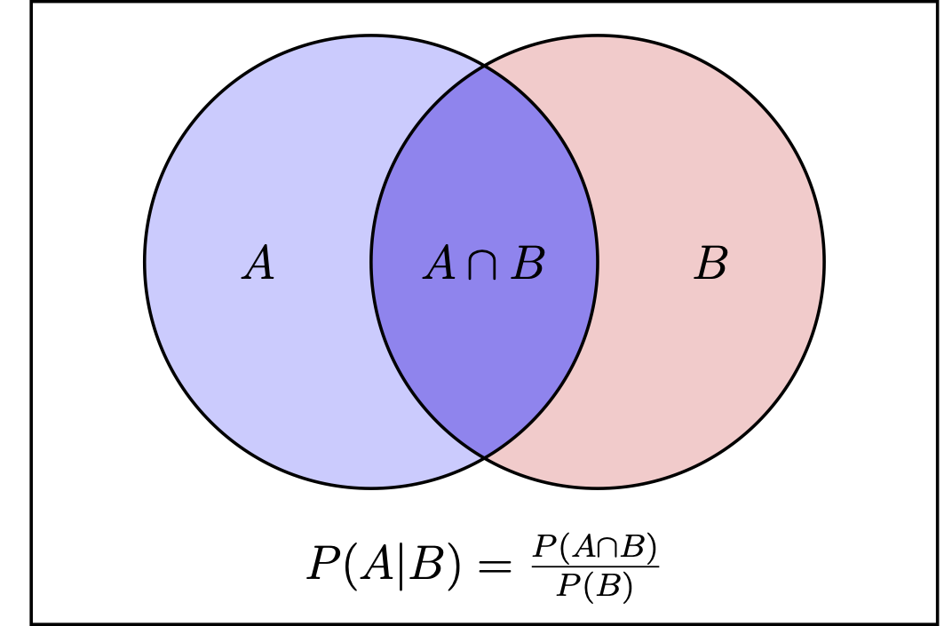
In this lecture, we will look into a model called Naive Bayes. But, before we get into the nitty-gritty details of the model, we should first discuss some of the probability theory needed to understand it. Probability is the likelihood that an event occurs (which is normally estimated from the data available to us). If we want to calculate the probability that a person has a disease, then we could estimate the probability as \[P(\text{Disease}) = \frac{\#\text{ of observed people with disease}}{\text{total \# of people observed}}.\] We can note that having the two events of having the disease and not having the disease are mutually exclusive and exhaustive. Mutually exclusive refers to the fact that the two events can not occur at the same time, and exhaustive refers to the fact that these are the only two possible outcomes in the event space.
Imagine that there is some disease that affects \(3\%\) of the population. We could use this \(3\%\) probability to predict if someone has the disease, with this value being the prior probability. Now, imagine that there is a test that we can perform with \(95\%\) accuracy to see which individuals have the disease. If we are tested for the disease and the results come back positive (indicating we have the disease), does that mean we have a 95% chance of having the disease (since the test is 95% accurate)? Not quite… The actual probability of us having the disease after we test positive for the disease is actually around \(37\%\). We will see how we got this exact number shortly, but the main takeaway right now is that we came into the problem assuming we had a \(3\%\) chance of having the disease, which is the prior probability. After some new information (mainly testing positive for the disease) we are able to update our probability of having the disease to \(37\%\), which is our posterior probability.
To derive this calculation, we should review some basic properties of probability. To begin, if two events are independent then \(P(A\cap B) = P(A)\cdot P(B)\), where \(P(A\cap B)\) is the probability that events \(A\) and \(B\) occur at the same time. If two events are not independent then \(P(A\cap B) = P(A) \cdot P(B|A)\) where \(P(B|A)\) is the probability \(B\) occurs given \(A\) has occurred as well. This formula is the foundation of Bayes Theorem which deals with conditional probability (probability of \(A\) conditioned on the fact \(B\) also occurs): \[P(A|B) = \frac{P(A \cap B)}{P(B)}\]
Manipulating the equation and using the fact that \(P(A\cap B) = P(B \cap A)\) gives us: \[\begin{align*}
P(A|B) =& \frac{P(A\cap B)}{P(B)} \\
P(A|B)\cdot P(B) =& P(A \cap B) = P(B \cap A) = P(B|A) \cdot P(A) \\
P(A|B) =& \frac{P(B|A)\cdot P(A)}{P(B)}
\end{align*}\] In the case above, \(P(A)\) is the prior probability, and \(P(A|B)\) is the posterior probability (updated now that we know \(B\) has also occurred).
So, going back to our medical example we can calculate the probability of having the disease given we test positive for it, which is \(P(\text{Disease} | \text{Positive Test})\). \[P(\text{Disease} | \text{Positive Test}) = \frac{(\text{Positive Test} | \text{Disease}) \cdot P(\text{Disease})}{P(\text{Positive Test})}\]
We know the prior probability of having the disease is \(3\%\), meaning \(P(\text{Disease}) = 0.03\). We also know that the test is \(95\%\) accurate, so if we have the disease the test will identify it \(95\%\) of the time, meaning \(P(\text{Positive Test}|\text{Disease}) = 0.95\). We could also easily calculate the probability of testing positive by looking at the proportion of people who have the disease and correctly test positive for it along with the proportion of people who do not have the disease and falsely test positive for it. This would give us:
Therefore, one can calculate the probability an individual has the disease given they have tested positive as: \[P(\text{Disease} | \text{Positive Test}) = \frac{(0.03 \cdot 0.95)}{(0.03 \cdot 0.95) + (0.97 \cdot 0.05)} = \frac{0.0285}{0.077} = 0.3701299 \approx 37\%\]
This may seem “off” to us at first, as we claim the test is \(95\%\) accurate, but the test is also labeling people who do not have the disease (a majority of the population) as having it. So, we have to determine the proportion of people who have it and tested positive out of the total number who tested positive. Using the new information that we tested positive, we have updated our probability of having the disease from \(3\%\) to \(37\%\), and if an additional test is run showing a positive result it would update our probability of having the disease to \(92\%\).
There are two main schools of thought in statistics: Frequentist (probabilities are fixed and unchanging) and Bayesian (probabilities can be updated with new information). The idea of conditional probability and the Bayesian way of thinking (updating our probabilities as new information becomes available to us) is important for a variety of machine learning models. The math shown above was to give you context into Bayesian statistics and some of the theories that the Naive Bayes model relies on.
10.2 The Naive Bayes Classifier
Let us look at an example of trying to classify an email as “Spam” or “Ham” (not Spam). We look at 100 emails and notice that \(20\%\) of them are spam. We decide that we want to calculate the probability an email is “Spam” given the words “FREE!!” are within the email. Below is a contingency table which describes the occurrences of “FREE!!” within the emails:
Before we do any calculations to determine if an email containing the word “FREE!!” is “Spam” or “Ham”, we can notice that \(P(\text{FREE!!}|\text{Spam})=4/20\), \(P(\text{Spam})=20/100\), \(P(\text{FREE!!})=5/100\), and \(P(\text{FREE!!} \cap \text{Spam}) = 4/100\). Looking at the contingency table we could probably quickly calculate \(P(\text{Spam}|\text{FREE!!})\) as \(4/5\). This would indicate that the email is “Spam”. We could also calculate it using our formula and arrive at the same conclusion: \[P(\text{Spam}|\text{FREE!!}) = \frac{P(\text{FREE!!}|\text{Spam}) \cdot P(\text{Spam})}{P(\text{FREE!!})} = \frac{0.2 \cdot 0.2}{0.05} = 0.8\]
We can expand on this idea and attempt to determine if an email is “Spam” or “Ham” by including the words “FREE!!!” (denoted as \(W1\)), “guarantee” (\(W2\)), “satisfaction” (\(W3\)), and “warranty” (\(W4\)) in our model. So, say we have an email which contains the words “FREE!!” and “guarantee”, but does not include the other two words and we want to determine if it is spam or not. Therefore, we want to determine \(P(\text{spam} | W1 \cap W2 \cap !W3 \cap !W4)\). Reducing this conditional probability formula is extremely complex, so we will make a naive assumption and assume that all features are equally important and independent of each other. This assumption will rarely be true though, but Naive Bayes still performs well even when the features are not independent, so, as Data Scientists we will be able to sleep at night even knowing it is “good enough” (the pure mathematicians might cringe at this hand waving process though).
Below are tables showing us the data pertaining to each of the three new words being added to our model. Notice that the marginal sums are not included in these tables, but it is easy to calculate on our own:
Since we are making naive assumptions and assuming independence, we can break the conditional probability apart. Note that in the formula below, \(\propto\) means “proportional to” so therefore we are not calculating the actual probability. We will compare it to the other outcomes in the event space to determine its classification:
Likewise, we can calculate the probability of the email being “Ham” as follows: \[\begin{align*}
P(\text{ham} | W1 \cap W2 \cap & !W3 \cap !W4) \propto\\
& P(W1|\text{ham}) \cdot P(W2|\text{ham}) \cdot P(!W3|\text{ham}) \cdot P(!W4|\text{ham}) \cdot P(\text{ham}) \\
=& (1/80) \cdot (14/80) \cdot (71/80) \cdot (57/80) \cdot (80/100) = 0.001
\end{align*}\]
Therefore, we could classify an email containing the words “FREE!!” and “guarantee” but excluding the words “satisfaction” and “warranty” as “Spam”. Now imagine we received an email with all four words present. We could calculate the probabilities as:
This result is not what we would expect, as the email contains words that are typically associated with “Spam”. This likely incorrect classification is due to our naive assumptions and the fact one of the events is “rare” (we do not have a “spam” occurrence containing the word “satisfaction”). To try and tweak for rare events we can add a Laplace estimator into the model. All this will do is add a small value to each count in the frequency table so that no observation occurs 0 times (and thus makes the whole probability 0). This results in a classification of “Spam” since the probability is larger than the “Ham” classification. We can see this calculation below when we added 1 to each count in the frequency table:
The Naive Bayes model is beneficial in that it is relatively simple, fast, and very effective. It can classify both binary and multi-level classifications. We do not have the same concern with missing or noisy data as we did when we performed linear or logistic regression. This model is also beneficial because we can train our model with relatively few examples, but it can also handle a large number of observations as well. A downside to this model is that it is not ideal for datasets with many quantitative features. Also, the estimated probabilities are less reliable (since we only calculated the proportionality) than the predicted class.
As we get ready to run the Naive Bayes model in R, we will need to prepare our data. This is because the model requires the data to be categorical values converted to factors. If needed, we may need to use the cut() function to convert quantitative values into categorical levels using different bins. Be careful though, as too many bins will lead to an overfitting of the model and too few bins will lead to an underfitting of the model.
10.5 Building a Naive Bayes Model in R
To see the Naive Bayes model worked out in R, we will look at the titanic_train dataset found in the titanic library. We used this same dataset when we were using logistic regression to predict is passengers would survive or not. So, the first thing we will need to do is to transform the data by converting some variables to factors and in one case converting a quantitative variable into a categorical variable. Note that this may be “neater” to do using dplyr or tidyr, but Dr. McCurdy thinks it is just as easy to alter the dataset this way:
  Survived Pclass    Sex Age_C
1       No      3   male Adult
2      Yes      1 female Adult
3      Yes      3 female Adult
4      Yes      1 female Adult
5       No      3   male Adult
7       No      1   male Adult
We can then randomly partition the data into a training and testing set with both the predictor variables and the outcome variables. We have also saved the training classification and the testing classification as an additional vector to be used later.
To create a Naive Bayes model, we will need to install and call the e1071 library. The naiveBayes() function will allow us to create a model much like we did when we built our linear regression models. The function also allows us to specify if a Laplace estimator is to be included in the model:
Naive Bayes Classifier for Discrete Predictors

Call:
naiveBayes.default(x = X, y = Y, laplace = laplace)

A-priori probabilities:
Y
       No       Yes
0.5814361 0.4185639

Conditional probabilities:
     Pclass
Y             1         2         3
  No  0.1596386 0.1927711 0.6475904
  Yes 0.4016736 0.3012552 0.2970711

     Sex
Y        female      male
  No  0.1415663 0.8584337
  Yes 0.6778243 0.3221757

     Age_C
Y         Adult     Child
  No  0.8674699 0.1325301
  Yes 0.7824268 0.2175732
After we have built the model, we can use it to predict what each categorical outcome would be. It should be noted that the model itself also provides us with the prior probabilities and conditional probabilities. If we wanted (which we probably don’t), we could calculate the probability of our observation surviving or not surviving. Luckily though, this can be done using the predict() function along with passing in the model and test data.
pred <-predict(mod, test)head(pred)
[1] Yes Yes No  Yes Yes No
Levels: No Yes
table(orig,pred)
     pred
orig  No Yes
  No  75  17
  Yes 15  36
Finally, we can see above (and below) the confusion matrix which indicates how good (or bad) our model is. An accuracy rate of \(77.62\%\) is roughly what we had when we ran logistic regression. Within the confusionMatrix() function we can set the mode argument to show all available metrics. This way we can see all the metrics that were discussed in previous lectures such as precision, recall, specificity, and sensitivity.