library(ISLR)
set.seed(11)
train_indices <- sample(1:nrow(Auto), nrow(Auto)*.80)

Autotrain <- Auto[train_indices,]
Autotest <- Auto[-train_indices,]

plot(Auto$weight, Auto$mpg, pch=20)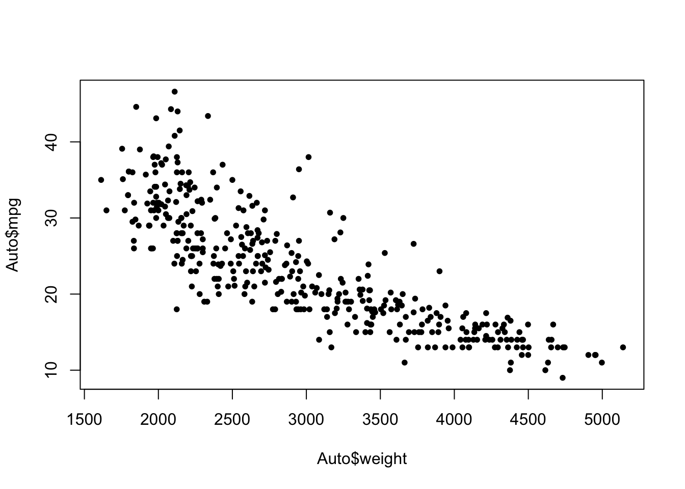
Throughout the course so far, we have been evaluating our model by seeing how well it describes the data that it uses to build the model. This is not ideal as our model has “memorized” this data already, so it will do reasonably well. This can lead to overfitting and inflated performance metrics, which will give us a false sense of how well the model does. To avoid this, we will want to see how our model does on new unseen data, and to do this we will introduce the idea of testing and training.
The general idea is to randomly break the dataset into two groups; one for training the model (roughly 75-80% of the data) and one for testing the model (the remaining data). The training set will be used to train the model (…go figure), where we will adjust parameters and try to choose the best model that captures the underlying relationship of the data. After we think we have found an acceptable model, we will use the testing set to test the model (…go figure again) and see how it does with this new data. A model that performs well on the test data implies it can generalize beyond the specific data learned in the training phase. A model that performs poorly on the test data likely implies the training model is overfitting the data instead of learning general patterns. It is important that we never train the model using the test set, as this data should only be used once to evaluate the performance of the model.
library(ISLR)
set.seed(11)
train_indices <- sample(1:nrow(Auto), nrow(Auto)*.80)
Autotrain <- Auto[train_indices,]
Autotest <- Auto[-train_indices,]
plot(Auto$weight, Auto$mpg, pch=20)
Looking at the output below, we can try a variety of different models and notice that the RMSE is the smallest for model 2 (where weight is raised to the \(-0.5\) power). After we select the model we think is best, we can use the predict() function to determine the predicted values in the testing set and then compare them to the actual values. We can see the RMSE of the test set is roughly 4.16. There is no ideal difference between the training set and the testing set that tells us it is a good model. We will just want to look for similar values. When the training RMSE \(\ll\) testing RMSE (where \(\ll\) means much lesser than) we will be overfitting the training data and when the training RMSE \(\gg\) testing RMSE we will be underfitting the training data.
model1 <- lm(mpg ~ weight, data=Autotrain)
sqrt(mean(model1$residuals^2))
[1] 4.288783model2 <- lm(mpg ~ I(weight^-0.5), data=Autotrain)
sqrt(mean(model2$residuals^2))[1] 4.18172model3 <- lm(mpg ~ I(weight^-1), data=Autotrain)
sqrt(mean(model3$residuals^2))[1] 4.241288test_pred <- predict(model2, newdata=Autotest)
sqrt(mean((test_pred - Autotest$mpg)^2))[1] 4.159494While this process is good and helps us avoid building the model solely for the training set, it does only give us one chance at testing the model. To get around this, we can create a third set of data called the validation set (with a potential breakdown of the different sets being 60% train, 20% validation, 20% test). With this, we can train our data and then use the validation set to get a glimpse of what the testing performance may be. Remember, we can only use the testing set once since this is new and unseen data, but we can use the validation set many times. This validation set will allow us to tune, test, and select the best model without ever touching the testing set.
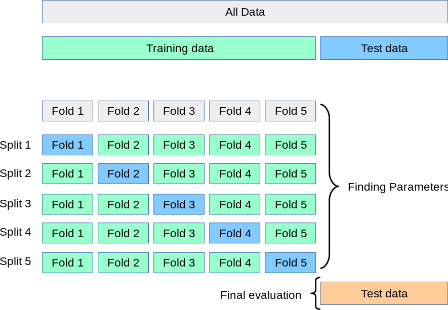
As an astute data science practitioner, you may be asking the questions: “What if I get an unlucky split?”, or “What if there is an extreme value in one of my sets?”, or even “What if I have a small dataset and there are not many values in each group?”. These are all issues that will impact the model training and evaluation. To address some of these issues, we will introduce the concept of \(k\)-fold Cross-Validation. With this method, we will break the training set into \(k\) groups. A model is trained \(k\) times, each time using \(k-1\) folds for training and 1 fold for validation. This way each group is used to validate the model. We could then estimate the test RMSE by averaging the \(k\) validation set RMSEs. After determining which model should be used, we can then build the model using the whole training set and then determine its performance using the testing set. The idea of the process can be seen below. There are libraries in R which will help you do this more efficiently:
library(caret)
# Using the same train/test set we made previously:
folds <- createFolds(Autotrain$mpg, k = 5, list = TRUE)
results <- c()

for(i in 1:5){
  train <- Autotrain[-folds[[i]],]
  validate <- Autotrain[folds[[i]],]
  model <- lm(mpg ~ I(weight^-0.5), data = train)
  preds <- predict(model, validate)
  RMSE <- sqrt(mean((preds - validate$mpg)^2))
  results <- c(results, RMSE)
}

results # RMSE of Validation Set for each Fold
[1] 5.027488 4.393549 4.158359 3.149976 4.095175mean(results) # Mean RMSE will approximate Test RMSE[1] 4.164909model1 <- lm(mpg ~ I(weight^-0.5), data=Autotrain)
test_pred <- predict(model1, newdata=Autotest)
sqrt(mean((test_pred - Autotest$mpg)^2))[1] 4.159494We would want to use Cross-Validation (CV) to determine which model should be built. We will then build the model using the whole training dataset. Notice how the CV RMSE is a very good estimator of the test RMSE.
As we are talking about different models and over/underfitting, we should take a second to quickly discuss bias and variance (and the trade-off between the two). Bias is essentially how well our model fits the training data while Variance is how sensitive the model is to small changes in the training set. While there are equations to calculate the bias and variance of a model, we will focus on the idea of how the bias and variance will change when our model becomes more or less complex (flexible). We will want to find the sweet spot where our model does not underfit or overfit the data. Below is a visualization that visualizes the trade-off between the two metrics:
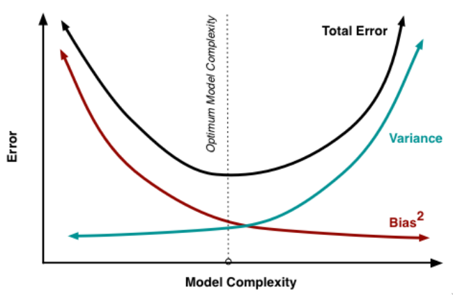
As our model becomes more complex/flexible (think adding more exponent terms) the Bias will decrease. This makes sense because as we know when we add more terms into the model it will better model the training data and raise the \(R^2\) value. If we have a model with many terms in it, then a slight adjustment to the training data would result in a wildly different model, resulting in a large Variance. On the flip side, if we have a rigid model (maybe with only one term) then it might not fit the training data very well, resulting in a large Bias. However, the rigid model will also be immune to slight changes in the training data since it is very basic, resulting in a low Variance. The goal for us will be to try and find the sweet spot where the Bias and Variance are minimized (this spot will be different for every dataset/model).
As we are building our model, we should note that there are a few different ways to determine how complex the models should be. The first way we will discuss is to use the Partial F-Test to help us decide if adding a term is beneficial to the model. This test allows us to compare nested models (same features but an additional one is included) using the anova() function. The null hypothesis will be that the Fit between the 2 models is equal and the alternative hypothesis is that Fit is improved with the more complex model.
\[H_0: \text{Fit between 2 models is equal} \quad \text{vs} \quad H_A: \text{Fit is improved with more complex model}\]
model1 <- lm(mpg ~ 1, data=Auto)
model2 <- lm(mpg ~ weight, data=Auto)
model3 <- lm(mpg ~ weight + horsepower, data=Auto)
model4 <- lm(mpg ~ weight + horsepower + displacement, data=Auto)
anova(model1, model2, model3, model4)
Analysis of Variance Table
Model 1: mpg ~ 1
Model 2: mpg ~ weight
Model 3: mpg ~ weight + horsepower
Model 4: mpg ~ weight + horsepower + displacement
Res.Df RSS Df Sum of Sq F Pr(>F)
1 391 23819.0
2 390 7321.2 1 16497.8 917.0641 < 2.2e-16 ***
3 389 6993.8 1 327.4 18.1986 2.503e-05 ***
4 388 6980.0 1 13.8 0.7682 0.3813
---
Signif. codes: 0 '***' 0.001 '**' 0.01 '*' 0.05 '.' 0.1 ' ' 1Looking at the four models, we can notice that they are nested since each model adds one new feature. The first model contains just the intercept with no quantitative predictor. The output shows us that the second model is an improvement from the first model (due to the low p-value). Additionally, the third model is a statistical improvement from the second model, implying this model with 2 quantitative features is a better fit than the model with just 1 quantitative feature. Finally, the fourth model does not result in an improved fit over the third model, meaning it does not bring any added benefit to the model.
Another way to evaluate a model is to use a Criterion-Based Selection metric. This method does not require nested models and allows us to compare models with different features. We will prefer the model with the lower criterion value. The two main criterion metrics are Akaike’s Information Criterion (AIC) and the Bayesian Information Criterion (BIC). We will not bother ourselves with the formulas for these, but we should know that both of these rewards the goodness of fit while penalizing model complexity. It should be noted that the two metrics will not always result in the same “ideal” model being recommended.
AIC(model1, model2, model3, model4) df AIC
model1 2 2726.383
model2 3 2265.939
model3 4 2250.005
model4 5 2251.230BIC(model1, model2, model3, model4) df BIC
model1 2 2734.325
model2 3 2277.852
model3 4 2265.890
model4 5 2271.086The last thing that we will discuss in this lecture is how we can determine which features are important enough to include in the model. There are several ways this can be done, with the two main methods being Forward Selection and Backward Selection. Forward selection starts will a null model (no predictors) and adds the feature which results in a one-variable model with the lowest RSS (or a predictor that is the “most significant”, or the lowest AIC, etc.). We then keep adding predictors one at a time, looking at all possible additions, and only stop until some criterion is met (AIC rising, no more statistically significant additions, etc).
The Backward selection method starts with a full model (all of the predictor variables) and removes a non-significant predictor variable with the largest \(p\)-value. It then runs the model again until only significant predictor variables are left. There is also a method that does both forward and backward, adding predictors and if the addition of one makes a different variable non-significant it will remove it. It should be noted that each method may result in a different model being built.
Luckily, this can be done in R using the regsubsets() function in the leaps library. The user can specify the method as forward, backward, or exhaustive. When looking at the summary, wherever there is an asterisk (*). An example of this can be seen below, with some of the output edited to fit onto the page. It tells us the best 1-variable model includes CRBI, while the best 2-variable model includes CRBI and Hits. Notice how when using the exhaustive method some of the variables become significant, lose significance, and then become significant again (AtBat,CAtBat, CRBI, etc.). Also notice how different methods result in different results, so depending on which method you use you will get different 7-variable models.
library(leaps)
Hitters1 <- Hitters[,c("Salary","AtBat", "Hits", "Walks", "CAtBat",
                       "CHits", "CHmRun", "CRuns", "CRBI", "CWalks",
                       "Division", "PutOuts")]
model1 <- regsubsets(Salary ~ ., Hitters1,
                     method="exhaustive", nvmax=12)
summary(model1)$adjr2
[1] 0.3188503 0.4208024 0.4450753 0.4672734 0.4808971 0.4972001 0.5007849
[8] 0.5137083 0.5180572 0.5170636 0.5151403model2 <- regsubsets(Salary ~ ., Hitters1,
method="forward", nvmax=12)
summary(model2)Subset selection object
Call: regsubsets.formula(Salary ~ ., Hitters1, method = "forward",
nvmax = 12)
11 Variables (and intercept)
Forced in Forced out
AtBat FALSE FALSE
Hits FALSE FALSE
Walks FALSE FALSE
CAtBat FALSE FALSE
CHits FALSE FALSE
CHmRun FALSE FALSE
CRuns FALSE FALSE
CRBI FALSE FALSE
CWalks FALSE FALSE
DivisionW FALSE FALSE
PutOuts FALSE FALSE
1 subsets of each size up to 11
Selection Algorithm: forward
AtBat Hits Walks CAtBat CHits CHmRun CRuns CRBI CWalks DivisionW
1 ( 1 ) " " " " " " " " " " " " " " "*" " " " "
2 ( 1 ) " " "*" " " " " " " " " " " "*" " " " "
3 ( 1 ) " " "*" " " " " " " " " " " "*" " " " "
4 ( 1 ) " " "*" " " " " " " " " " " "*" " " "*"
5 ( 1 ) "*" "*" " " " " " " " " " " "*" " " "*"
6 ( 1 ) "*" "*" "*" " " " " " " " " "*" " " "*"
7 ( 1 ) "*" "*" "*" " " " " " " " " "*" "*" "*"
8 ( 1 ) "*" "*" "*" " " " " " " "*" "*" "*" "*"
9 ( 1 ) "*" "*" "*" "*" " " " " "*" "*" "*" "*"
10 ( 1 ) "*" "*" "*" "*" "*" " " "*" "*" "*" "*"
11 ( 1 ) "*" "*" "*" "*" "*" "*" "*" "*" "*" "*"
PutOuts
1 ( 1 ) " "
2 ( 1 ) " "
3 ( 1 ) "*"
4 ( 1 ) "*"
5 ( 1 ) "*"
6 ( 1 ) "*"
7 ( 1 ) "*"
8 ( 1 ) "*"
9 ( 1 ) "*"
10 ( 1 ) "*"
11 ( 1 ) "*" If you were to do this again but choose the backward method you will see that it gives different results as well. I would recommend the exhaustive method as it checks for all possible combinations. In addition to the methods already discussed, there are additional ones such as Step-wise AIC which we will not discuss here, but it has a similar setup to what we have already learned. I will end off the lecture by reminding you that the simpler model (if the metrics are similar) is usually preferred over the complicated one. Model and Feature selection is as much an art as it is a science.