So far throughout the course, most of the models we have discussed have been examples of supervised learning. This means that we have an outcome variable that we are trying to predict, and we use the observed outcome values to help train the model. For example, with linear regression we may know the price of a house and try to predict that price using characteristics of the house, and with KNN we may know the species of a flower and use nearby flowers to classify a new observation. But, what happens if there is no outcome variable and we just want to see if there are natural groups hidden within the data?
This type of problem falls under the umbrella of unsupervised learning. Instead of trying to predict a known outcome, we are interested in finding structure within the predictor variables themselves. One of the most common examples of unsupervised learning is clustering, where we attempt to group observations that are similar to each other. There are many possible clustering algorithms, but we will begin with one of the most approachable methods: K-Means Clustering.
A common application might be customer segmentation. Imagine we have information about how much customers spend, how often they shop, and how long they have been customers. We may not have a variable telling us which “type” of customer each person is, but perhaps there are natural groups in the data. We may find one group of frequent low-spending customers, another group of occasional high-spending customers, and another group somewhere in between. K-Means will try to identify these groups for us.
14.1 Supervised vs. Unsupervised Learning
Before we discuss exactly how K-Means works, we should distinguish clustering from the classification methods we have already seen. With classification, we are given the correct classes while training the model. With clustering, those classes do not exist ahead of time.
Method
Outcome Known?
Main Goal
Linear Regression
Yes
Predict a quantitative value
Logistic Regression
Yes
Predict a binary outcome
KNN
Yes
Predict a categorical outcome using nearby observations
K-Means
No
Group similar observations together
In KNN, \(K\) refers to the number of nearby observations we use to classify a new observation. In K-Means, \(K\) refers to the number of clusters we want the algorithm to find. KNN already knows the classifications of the training observations, while K-Means is trying to discover groups without being given any classifications.
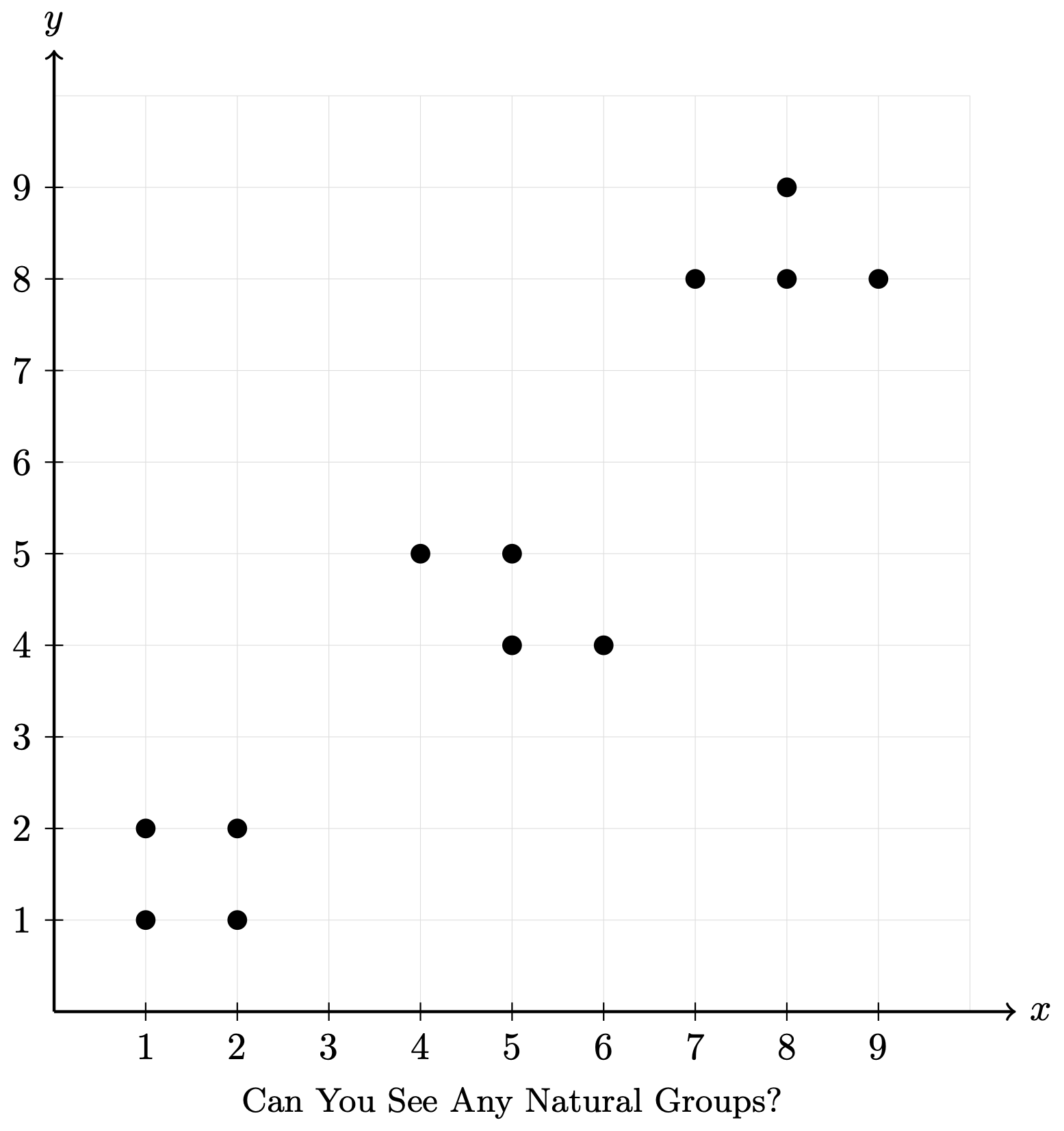
For instance, suppose we have the following data:
Without being told anything else about these points, we might look at the plot and decide that there appear to be three groups. There is a group toward the bottom left, another near the center, and another toward the upper right. The goal of K-Means is essentially to formalize this process so the computer can decide which observations should be placed together, as high dimensional data will be impossible for us humans to do by just looking at it.
The main question then becomes: what do we mean when we say two observations are “similar”? Much like with KNN, we will define similarity using distance. For two-dimensional data, the Euclidean distance between an observation \((x_i,y_i)\) and the center of a cluster \((\bar{x}_c,\bar{y}_c)\) can be written as
The notation may look a little intimidating, but all we are really doing is finding the straight-line distance between the observation and the center of the cluster. We already encountered this same general idea when discussing KNN.
14.2 How the K-Means Algorithm Works
The K-Means algorithm has a fairly simple objective: place observations into \(K\) clusters so that observations within the same cluster are as close to each other as possible. Each cluster will have a centroid, which is the mean location of all observations assigned to that cluster. The algorithm then repeatedly moves observations and centroids until the groups stop changing.
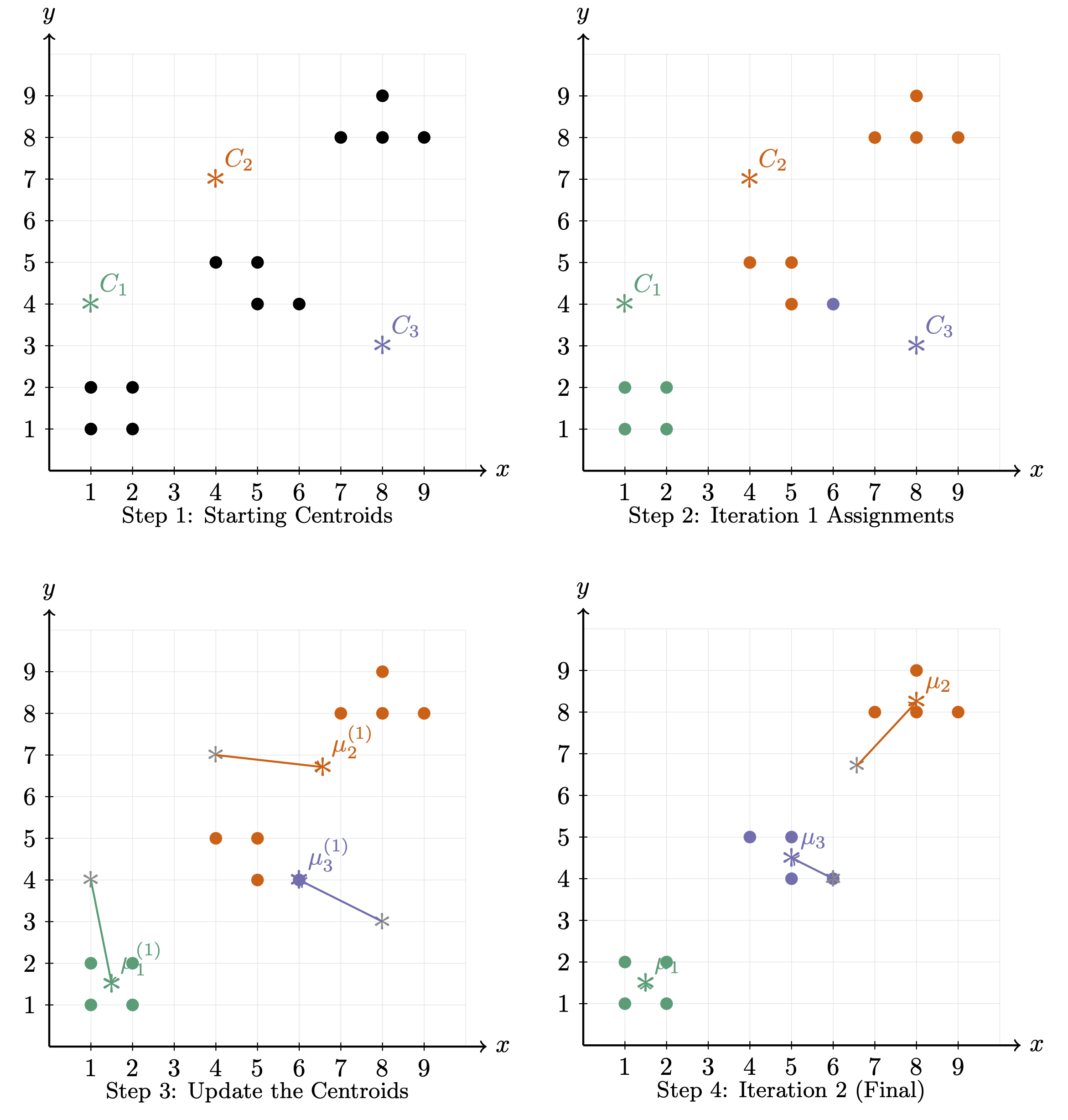
The general process is:
Choose the number of clusters, \(K\).
Select \(K\) starting centroids randomly.
Assign every observation to the closest centroid.
Recalculate each centroid using the mean of the observations assigned to that cluster.
Repeat steps 3 and 4 until the cluster assignments no longer meaningfully change.
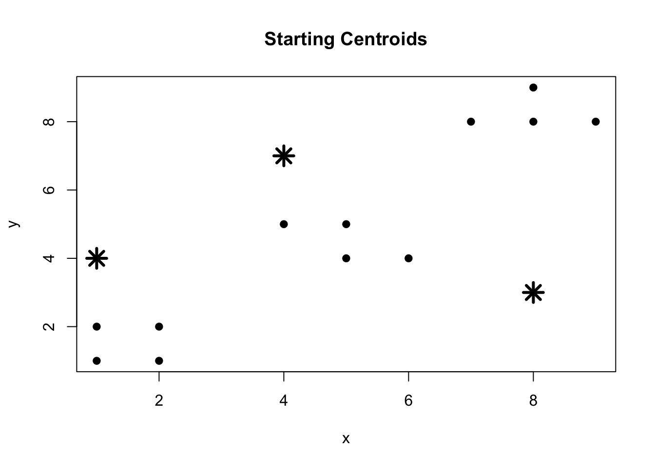
Let us use the small dataset from above and select three initial centers. These are intentionally not perfect centers because the whole point of the algorithm is that they will be updated.
For every observation, K-Means will calculate the distance to each of these three centers and assign the observation to whichever center is closest. For instance, we could manually calculate the distances from the first observation \((1,1)\) to each starting centroid:
point <-c(1,1)sqrt(sum((point - initial_centers[1,])^2))
[1] 3
sqrt(sum((point - initial_centers[2,])^2))
[1] 6.708204
sqrt(sum((point - initial_centers[3,])^2))
[1] 7.28011
The observation would be assigned to the cluster associated with the smallest of these three distances. After every observation has been assigned, we calculate a new mean \(x\) and mean \(y\) for each cluster. Those means become the new centroids, and then we repeat the process until the clusters do not change (this may take multiple iterations to settle down).
Luckily, we do not need to do all of these calculations manually. The kmeans() function in R will repeat the process for us until it converges.
K-means clustering with 3 clusters of sizes 4, 4, 4

Cluster means:
    x    y
1 1.5 1.50
2 8.0 8.25
3 5.0 4.50

Clustering vector:
 [1] 1 1 1 1 2 2 2 2 3 3 3 3

Within cluster sum of squares by cluster:
[1] 2.00 2.75 3.00
 (between_SS / total_SS =  95.8 %)

Available components:

[1] "cluster"      "centers"      "totss"        "withinss"     "tot.withinss"
[6] "betweenss"    "size"         "iter"         "ifault"
Notice that the cluster centers are not necessarily actual observations in the dataset. They are simply the means of the observations within each cluster. This is why we call the method K-Means (…the naming people did us a favor on this one).
The algorithm is trying to minimize the within-cluster sum of squares, which we will abbreviate as WCSS. This measures how far observations are from their own cluster center:
This idea should feel somewhat familiar. In regression we tried to find a line that minimized the squared residuals. Here, instead of measuring the vertical distance from an observation to a regression line, we are measuring the distance from an observation to its cluster centroid. We square these distances and try to make the total as small as possible.
We can access this information from the K-Means model:
toy_kmeans$withinss
[1] 2.00 2.75 3.00
toy_kmeans$tot.withinss
[1] 7.75
toy_kmeans$size
[1] 4 4 4
toy_kmeans$centers
    x    y
1 1.5 1.50
2 8.0 8.25
3 5.0 4.50
The withinss value tells us the within-cluster sum of squares for each individual cluster, while tot.withinss adds all of them together. The size output tells us how many observations were assigned to each cluster, and centers gives us the coordinates of the final centroids.
14.3 Running K-Means in R
Let us now move to a dataset we have encountered before. The iris dataset contains measurements of 150 flowers from three different species. We have previously used the species as an outcome variable for classification, but this time we are going to pretend that we do not know the species. We will only give the algorithm the four quantitative measurements and see whether it can discover natural groups on its own.
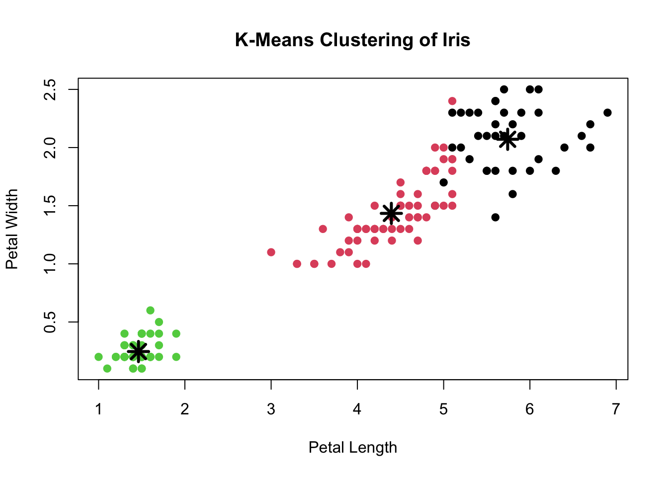
We happen to know that there are three species in the data, so we will begin by asking K-Means to create three clusters. The basic syntax is very simple: pass the quantitative data into kmeans() and specify the number of centers.
There are several important pieces of information in the output. The cluster means are stored in centers, the cluster assignment for each observation is stored in cluster, and the number of observations in each cluster is stored in size.
Even though we are only displaying two variables in the graph, remember that the model above used all four quantitative variables when deciding which observations belonged together, so that is why the observations might not appear to belong to the closest centroid.
Since we actually know the flower species, we can compare the clusters K-Means discovered with the true species after fitting the model. The species variable was not used by K-Means at all.
We should be careful when interpreting this table. Cluster 1 does not automatically mean virginica, Cluster 2 does not automatically mean versicolor, and so on. The numbers assigned to the clusters are arbitrary labels. If we ran the model again, the exact cluster numbers could switch even if the underlying groupings remained essentially the same.
What we should look for is whether the clusters line up reasonably well with the known species. We will usually see that setosa forms a very distinct group, while there is more overlap between versicolor and virginica. This makes sense if we look at the flower measurements, as setosa tends to be separated more clearly from the other species.
This example is useful because it lets us check how well the clusters correspond to a known grouping. In most real clustering problems though, we will not have a “correct” outcome variable sitting off to the side. If we already had that outcome variable, we would probably be doing classification instead!
There is one additional complication we should discuss before moving on. The K-Means algorithm begins with starting centroids, and different starting locations can sometimes produce different final clusters. This means that K-Means can settle on a solution that is good, but not necessarily the absolute best possible solution.
To reduce this issue, we can use the nstart argument. If we specify nstart=25, R will run K-Means 25 times using different starting centroids and keep the solution with the smallest total within-cluster sum of squares.
As a general rule, I would recommend using multiple starts rather than relying on a single random initialization. There is usually very little reason to trust one random starting point when R is perfectly willing to try several for us.
14.4 Scaling the Features
K-Means is a distance-based algorithm, which means the scale of the variables matters a great deal. We ran into the same issue with KNN. Suppose one feature ranges from 0 to 1 while another ranges from 0 to 10,000. A difference of 1 unit in the second variable is numerically much larger than a difference of 1 unit in the first variable, even though the first difference may be much more meaningful. The variable with the larger scale will tend to dominate the distance calculation.
A good example of this issue can be seen using the USArrests dataset, which contains violent crime statistics for the 50 states in 1973.
     Murder          Assault         UrbanPop          Rape
 Min.   : 0.800   Min.   : 45.0   Min.   :32.00   Min.   : 7.30
 1st Qu.: 4.075   1st Qu.:109.0   1st Qu.:54.50   1st Qu.:15.07
 Median : 7.250   Median :159.0   Median :66.00   Median :20.10
 Mean   : 7.788   Mean   :170.8   Mean   :65.54   Mean   :21.23
 3rd Qu.:11.250   3rd Qu.:249.0   3rd Qu.:77.75   3rd Qu.:26.18
 Max.   :17.400   Max.   :337.0   Max.   :91.00   Max.   :46.00
Notice that the variables are measured on very different scales. Assault, for example, is much larger numerically than Murder. If we perform K-Means directly on the raw data, the variables with the largest numerical scales will have the greatest influence on the clusters.
To avoid this problem, we can standardize each feature before clustering. A standardized value, or z-score, can be calculated as
\[z=\frac{x-\bar{x}}{s}.\]
This transforms every variable so that it has a mean of approximately 0 and a standard deviation of 1. Therefore, each variable begins on a comparable scale.
K-means clustering with 3 clusters of sizes 13, 20, 17

Cluster means:
      Murder    Assault   UrbanPop       Rape
1 -0.9615407 -1.1066010 -0.9301069 -0.9667633
2  1.0049340  1.0138274  0.1975853  0.8469650
3 -0.4469795 -0.3465138  0.4788049 -0.2571398

Clustering vector:
       Alabama         Alaska        Arizona       Arkansas     California
             2              2              2              3              2
      Colorado    Connecticut       Delaware        Florida        Georgia
             2              3              3              2              2
        Hawaii          Idaho       Illinois        Indiana           Iowa
             3              1              2              3              1
        Kansas       Kentucky      Louisiana          Maine       Maryland
             3              1              2              1              2
 Massachusetts       Michigan      Minnesota    Mississippi       Missouri
             3              2              1              2              2
       Montana       Nebraska         Nevada  New Hampshire     New Jersey
             1              1              2              1              3
    New Mexico       New York North Carolina   North Dakota           Ohio
             2              2              2              1              3
      Oklahoma         Oregon   Pennsylvania   Rhode Island South Carolina
             3              3              3              3              2
  South Dakota      Tennessee          Texas           Utah        Vermont
             1              2              2              3              1
      Virginia     Washington  West Virginia      Wisconsin        Wyoming
             3              3              1              1              3

Within cluster sum of squares by cluster:
[1] 11.95246 46.74796 19.62285
 (between_SS / total_SS =  60.0 %)

Available components:

[1] "cluster"      "centers"      "totss"        "withinss"     "tot.withinss"
[6] "betweenss"    "size"         "iter"         "ifault"
When we interpret the final clusters, though, standardized values are not always the easiest numbers to explain. It may be more meaningful to return to the original variables and calculate the average crime statistics within each cluster.
This output allows us to describe what makes each cluster different. For instance, one group may contain states with relatively low values across the crime variables while another may contain states with higher violent-crime measurements. The important part is that we are interpreting the clusters after the algorithm creates them. K-Means does not tell us that a group should be called “low crime” or “high crime”; those descriptions are ones we create by examining the characteristics of each cluster.
Since K-Means relies on Euclidean distance, I would typically recommend scaling quantitative variables unless there is a meaningful reason not to. If all variables are already measured on the same scale and a one-unit difference means roughly the same thing across variables, then scaling may not be necessary. But if the scales are substantially different, we should at least stop and think about it before running the model.
14.5 Choosing the Number of Clusters
So far we have conveniently told K-Means how many clusters to create. With iris, we knew there were three species, so using \(K=3\) was an obvious place to start. In a real unsupervised learning problem, however, the whole point may be that we do not know how many groups exist. This creates one of the most important questions in K-Means clustering: how do we choose K?
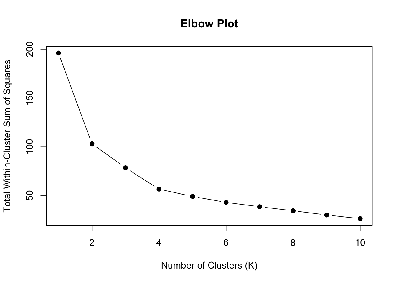
One possibility is to compare the total within-cluster sum of squares for several different values of \(K\). Remember that we want this value to be small because it means observations are close to their own cluster centers. Let us calculate the total within-cluster sum of squares for values of \(K\) from 1 through 10.
wss <-c()for(k in1:10){set.seed(101) model <-kmeans(USArrests_scaled, centers=k, nstart=25) wss[k] <- model$tot.withinss}wss
plot(1:10, wss, type="b", pch=19,xlab="Number of Clusters (K)",ylab="Total Within-Cluster Sum of Squares",main="Elbow Plot")
As \(K\) increases, the within-cluster sum of squares will always decrease. This makes sense because it becomes easier to keep observations close to a centroid when we are allowed to create more clusters. In the ridiculous extreme case where every observation had its own cluster, the within-cluster distance would be 0. That would technically minimize our WCSS, but it would not be a very useful clustering model.
Instead, we look for an elbow in the graph, which is where we see a big change in slope (this might be 2 or 4 for this graph). This is the point where adding another cluster stops producing a dramatic improvement in the within-cluster sum of squares. The graph may drop sharply at first and then begin to level off. The bend between those two patterns is a reasonable candidate for \(K\).
The elbow method is helpful, but it is not magic. Sometimes there is a very obvious elbow and other times the plot looks more like an arm without an elbow (…which is not especially useful to us). Therefore, we may want another method to help support our decision.
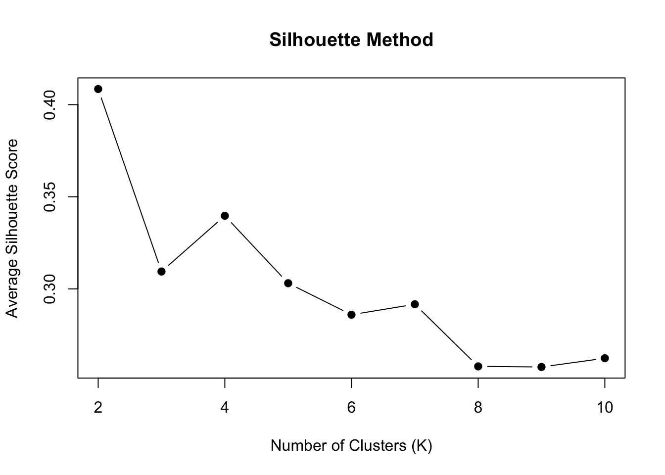
One option is the silhouette score. The silhouette score compares how close an observation is to the other observations in its own cluster with how close it is to observations in neighboring clusters. The value ranges from \(-1\) to \(1\).
A value close to \(1\) indicates the observation fits its own cluster well.
A value close to \(0\) indicates the observation is near the boundary between clusters.
A negative value indicates the observation may fit better in another cluster.
We can calculate the average silhouette score for several possible values of \(K\) using the cluster library.
library(cluster)silhouette_mean <-c()for(k in2:10){set.seed(101) model <-kmeans(USArrests_scaled, centers=k, nstart=25) sil <-silhouette(model$cluster, dist(USArrests_scaled)) silhouette_mean[k-1] <-mean(sil[,3])}silhouette_mean
plot(2:10, silhouette_mean, type="b", pch=19,xlab="Number of Clusters (K)",ylab="Average Silhouette Score",main="Silhouette Method")
With the silhouette method, larger values are preferred. Therefore, we might choose the value of \(K\) that produces the highest average silhouette score.
It is completely possible for the elbow method, silhouette score, and our practical interpretation of the clusters to suggest slightly different values of \(K\). This is not necessarily a problem. Unlike supervised learning, we often do not have a true outcome that tells us whether we are right or wrong. Choosing the number of clusters is partly a statistical question and partly an interpretation question.
14.6 Interpreting Clusters and Limitations
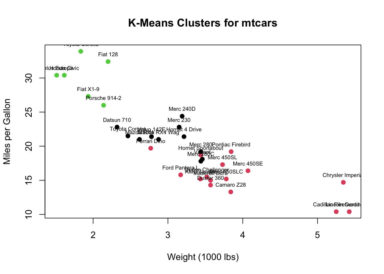
Let us finish with one more example using mtcars. We will cluster the cars based on fuel efficiency (mpg), horsepower (hp), weight (wt), and quarter-mile time (qsec).
Since horsepower, weight, fuel efficiency, and quarter-mile time are all measured on different scales, we should standardize the data before fitting the model.
The cluster numbers themselves are meaningless. There is nothing inherently “Cluster 1-ish” about the cars assigned to Cluster 1. Instead, we might examine the group averages and find a cluster of lighter, more fuel-efficient cars, another cluster of heavier and more powerful cars, and a third group somewhere between those extremes. We give the clusters meaning by examining the variables that characterize them.
K-Means is appealing because the underlying idea is fairly simple: group observations around the nearest mean. But, much like the other methods we have seen, most of the important decisions happen around the model rather than inside the function itself. We still need to decide which variables to include, whether they need to be scaled, how many clusters make sense, and whether the clusters tell us anything useful. The function can find the groups, but it is still our job as Data Scientists to decide what those groups mean.