plot(women$height, women$weight) 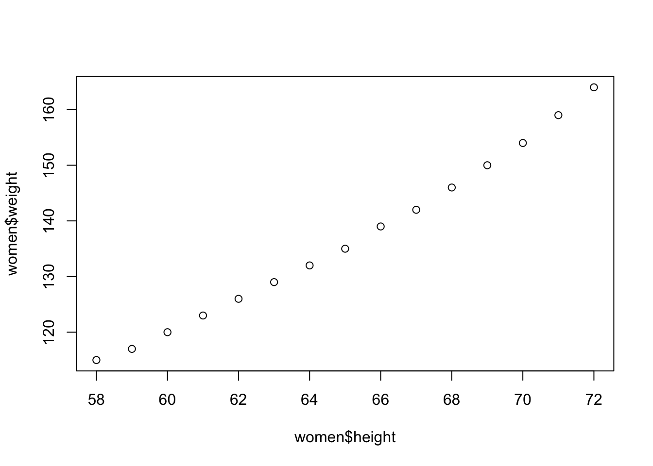
Throughout this course, we have seen several expansions for Simple Linear Regression. We have seen including categorical features, interaction terms, and additional quantitative features. In this lecture we will look at one last iteration of Linear Regression called Polynomial Regression. And yes, even though we will be dealing with polynomials it is still linear regression.
This type of regression will be beneficial if other linear models violate the assumptions of linearity and/or normality of the residuals. The idea for this will be to do a feature transformation (\(X^\lambda\)) with the most common values for lambda (\(\lambda\)) being -2, -1, -0.5, 0.5, 0, 1, 2, and sometimes 3. We will rarely use any other lambda transformation values as we will want to avoid over-fitting the model. To see this in action, let us look at an example in the women dataset where we can see a slight bend in the data:
plot(women$height, women$weight)
We can create a linear model to describe this relationship and we will see that based off this summary it is a very good model. This \(R^2\) value being .991 tells us that the model describes \(99.1\%\) of the variation in the data!!!
model1 <- lm(weight ~ height, data=women)
summary(model1)$r.square
[1] 0.9910098This would be a great model to use to make predictions, but it may not be a good model to use to explain the relationship between height and weight since the assumption (linearity) is violated when we look at the diagnostic plot of the data.
plot(women$height, women$weight)
abline(model1, col="red", lwd=2)
plot(model1, which=1)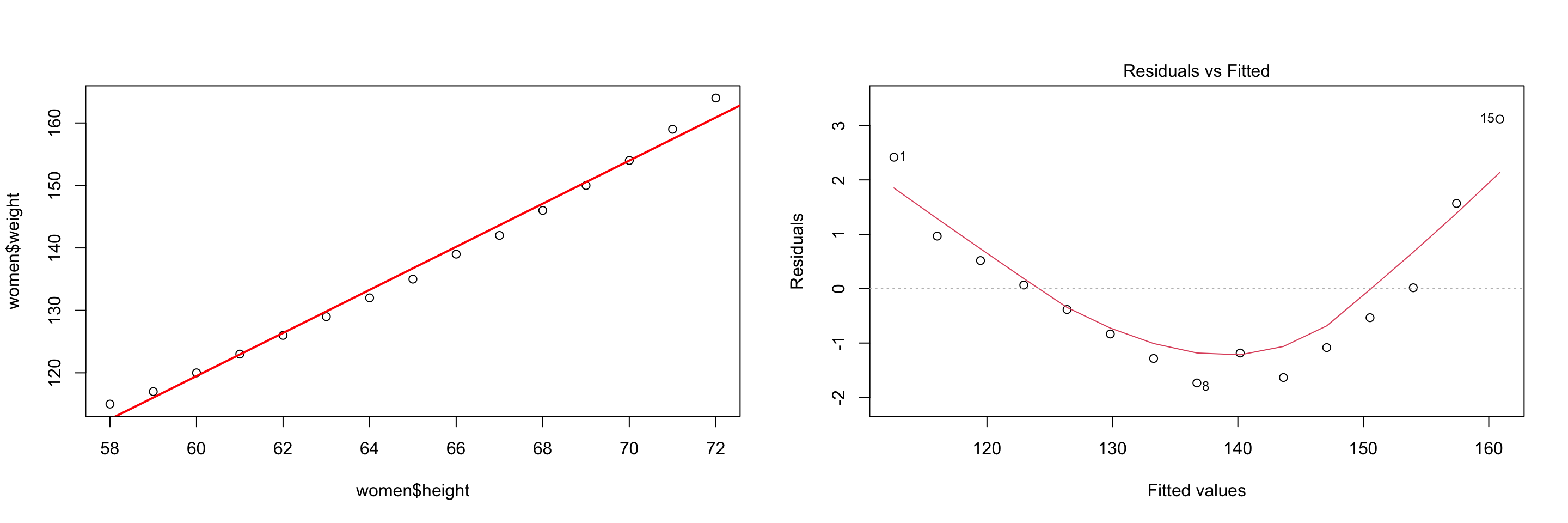
Based on this diagnostic plot, we can assume the data is not linear in nature and thus we might include a quadratic term. To include a quadratic term into the model we cannot just use \(\wedge\) since that by itself is used to deal with interaction terms (we did not explicitly mention it in the previous lecture, but \((hp + wt)^2= hp + wt + hp:wt\) within the model). To add a quadratic term in R, we will use the I() function to inhibit the interpretation of the command. This will make sense when we see it written below:
model2 <- lm(weight ~ height + I(height^2), data=women)
summary(model2)
Call:
lm(formula = weight ~ height + I(height^2), data = women)

Residuals:
     Min       1Q   Median       3Q      Max
-0.50941 -0.29611 -0.00941  0.28615  0.59706

Coefficients:
             Estimate Std. Error t value Pr(>|t|)
(Intercept) 261.87818   25.19677  10.393 2.36e-07 ***
height       -7.34832    0.77769  -9.449 6.58e-07 ***
I(height^2)   0.08306    0.00598  13.891 9.32e-09 ***
---
Signif. codes:  0 '***' 0.001 '**' 0.01 '*' 0.05 '.' 0.1 ' ' 1

Residual standard error: 0.3841 on 12 degrees of freedom
Multiple R-squared:  0.9995,    Adjusted R-squared:  0.9994
F-statistic: 1.139e+04 on 2 and 12 DF,  p-value: < 2.2e-16
\[\textbf{Model Equation: } \text{weight} = 261.88 + -7.35\times \text{height} + 0.08\times \text{height}^2\]
When we look at this model we can see it does even better in describing the variation of the data! Sure, some complexity was added to the model (something we would ideally want to avoid if possible) but the added terms are statistically significant, and the Adjusted \(R^2\) value increases. This model better explains the relationship between the two variables.
plot(women$height, women$weight)
x_values <- seq(min(women$height), max(women$height), length=20)
x_values <- data.frame(height = x_values)
y_pred <- predict(model2, newdata=x_values)
lines(x_values$height, y_pred, col="red", lwd=2)
plot(model2, which=1)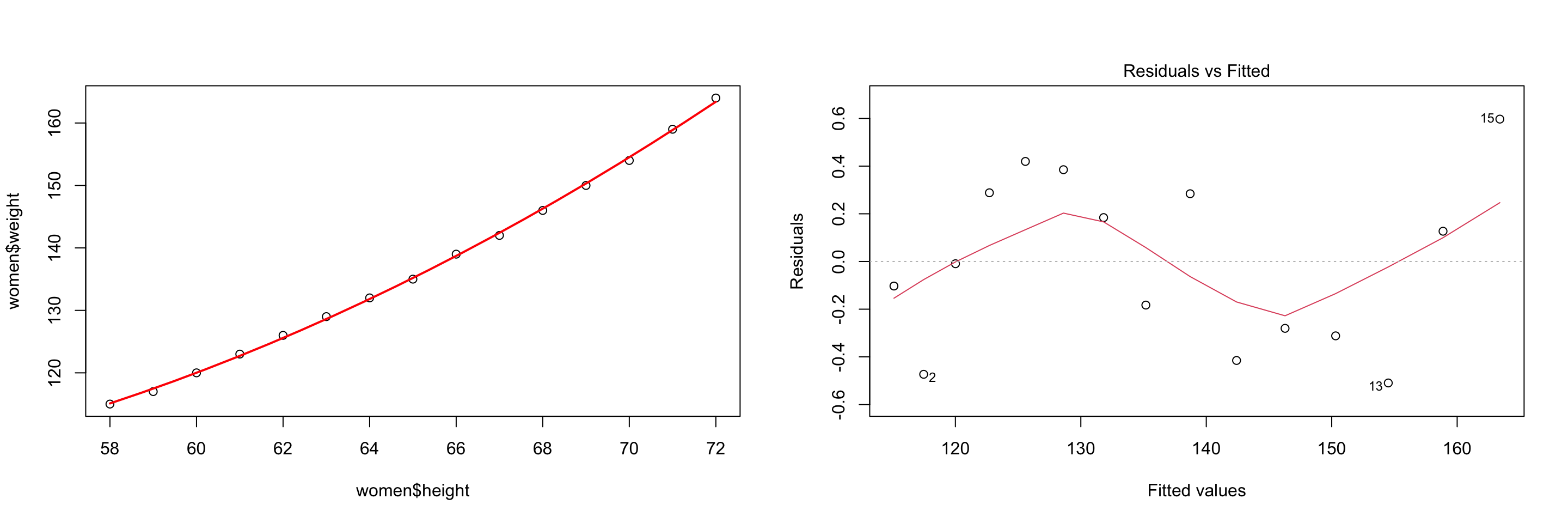
Looking at the model diagnostics, we can still see that there are still some issues with our fitted values and the residuals. Therefore, since the plot now looks like a cubic function we will add that term into the model and see how it affects it. As a note, we will always include the lower order terms (that is we will not do \(x + x^3\) without also including \(x^2\)).
model3 <- lm(weight ~ height + I(height^2) + I(height^3), data=women)
summary(model3)
Call:
lm(formula = weight ~ height + I(height^2) + I(height^3), data = women)

Residuals:
     Min       1Q   Median       3Q      Max
-0.40677 -0.17391  0.03091  0.12051  0.42191

Coefficients:
              Estimate Std. Error t value Pr(>|t|)
(Intercept) -8.967e+02  2.946e+02  -3.044  0.01116 *
height       4.641e+01  1.366e+01   3.399  0.00594 **
I(height^2) -7.462e-01  2.105e-01  -3.544  0.00460 **
I(height^3)  4.253e-03  1.079e-03   3.940  0.00231 **
---
Signif. codes:  0 '***' 0.001 '**' 0.01 '*' 0.05 '.' 0.1 ' ' 1

Residual standard error: 0.2583 on 11 degrees of freedom
Multiple R-squared:  0.9998,    Adjusted R-squared:  0.9997
F-statistic: 1.679e+04 on 3 and 11 DF,  p-value: < 2.2e-16
\[\textbf{Model Equation: } \text{weight} = -897 + 46.4\times \text{height} - 0.75 \times \text{height}^2 + 0.0043 \times \text{height}^3\]
This model seems to do an even better job of describing the data as the Adjusted \(R^2\) is even higher and all of the terms are statistically significant. If we look at a diagnostic of the model we can see that while there is still a slight pattern in the residual vs. fitted plot, it appears fairly “random”.
plot(women$height, women$weight)
x_values <- seq(min(women$height), max(women$height), length=20)
x_values <- data.frame(height = x_values)
y_pred <- predict(model3, newdata=x_values)
lines(x_values$height, y_pred, col="red", lwd=2)
plot(model3, which=1)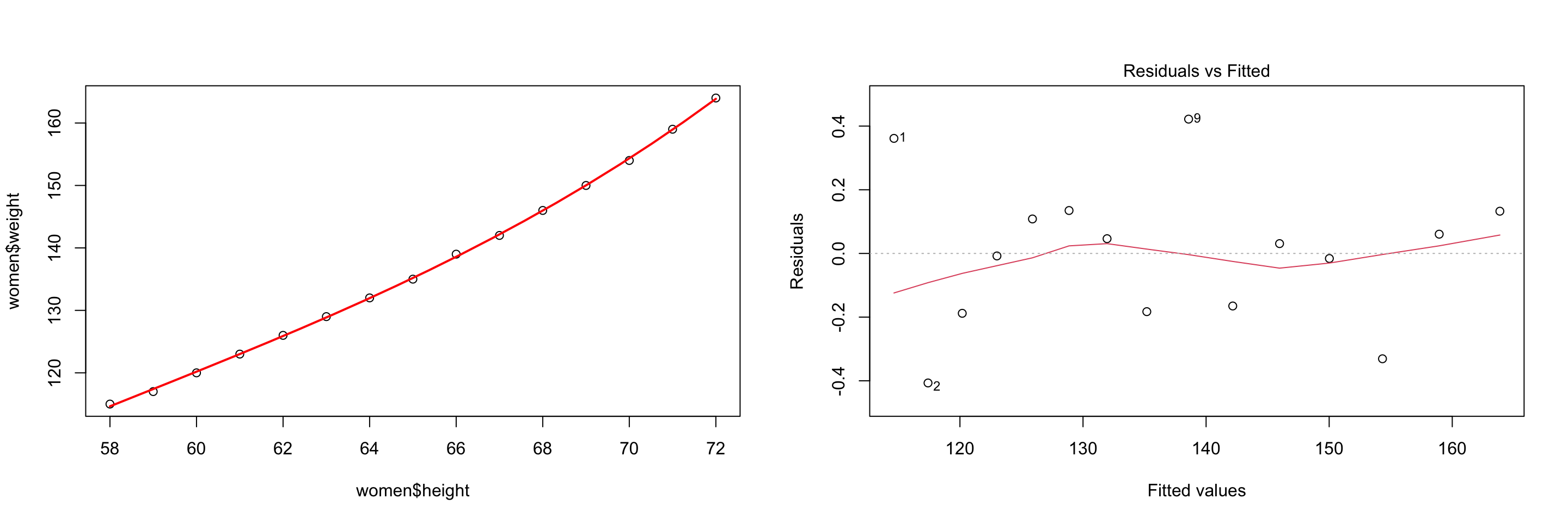
The main question we probably have right now is when we should stop adding powers to the models. Typically we will not go past the cubic transformation. We can use the boxTidwell() function in the car library to get an idea of what we should do. This will tell us the best-estimated value of \(\lambda\) along with if it is necessary (significant \(p\)-value). We will always round to the closest common value (mentioned at the beginning of this lecture). The code below says that a quartic (\(4^{th}\) power) model would be best, but we will stay using the cubic model for interpretation purposes.
library(car)
boxTidwell(weight ~ height, data=women)
MLE of lambda Score Statistic (t) Pr(>|t|)
4.2008 13.067 1.862e-08 ***
---
Signif. codes: 0 '***' 0.001 '**' 0.01 '*' 0.05 '.' 0.1 ' ' 1
iterations = 2 Let’s look at an example we have seen a few times previously and see the best way to model the data.
model1 <- lm(mpg ~ disp, data=mtcars)
summary(model1)$r.square
[1] 0.7183433par(mfrow=c(1,2))
plot(mtcars$disp, mtcars$mpg)
abline(model1, col="red", lwd=2)
plot(model1, which=1)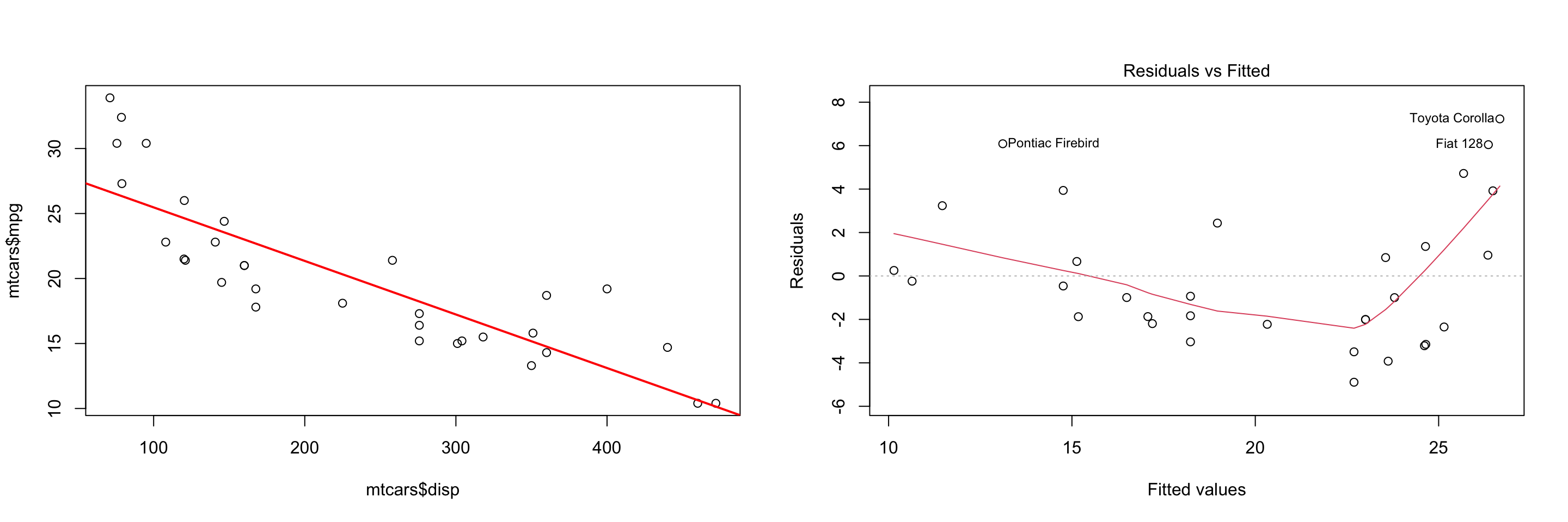
Based on the diagnostic plot, the linearity assumption is not met. We might try a quadratic model (raised to the second power) since the residuals look a little like it. But, we can also use the boxTidwell() function to get an idea of the type of transformation we should carry out. It informs us that an inverse transformation (raised to the \(-1\) power) is actually recommended, so we can build that within our lm() function without needing anything else written for the model.
boxTidwell(mpg ~ disp, data=mtcars) MLE of lambda Score Statistic (t) Pr(>|t|)
-0.90917 4.0194 0.0003796 ***
---
Signif. codes: 0 '***' 0.001 '**' 0.01 '*' 0.05 '.' 0.1 ' ' 1
iterations = 4 model2 <- lm(mpg ~ I(disp^-1), data=mtcars)
summary(model2)$r.square[1] 0.8596865To plot the line of best fit for this model we will use the predict function. You need to make sure that the name of the column in the dataframe is the exact same name as the variable in the model. The diagnostic plot looks better now since it has no discernible pattern.
plot(mtcars$disp, mtcars$mpg)
x_values <- seq(min(mtcars$disp), max(mtcars$disp), length=50)
x_values <- data.frame(disp = x_values)
y_pred <- predict(model2, newdata=x_values)
lines(x_values$disp, y_pred, col="red", lwd=2)
plot(model2, which=1)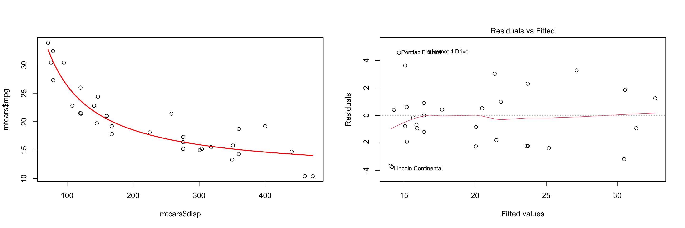
Looking at one more example with the boxTidwell() function, we can see the linear model with two predictors in the states dataframe has a fairly linear diagnostic plot. This indicates that we probably do not need to do any transformation on the predictors and the boxTidwell function confirms this:
states <- as.data.frame(state.x77[,c("Murder", "Population",
                                     "Illiteracy", "Income", "Frost")])
model1 <- lm(Murder ~ Population + Illiteracy, data=states)
plot(model1, which=1)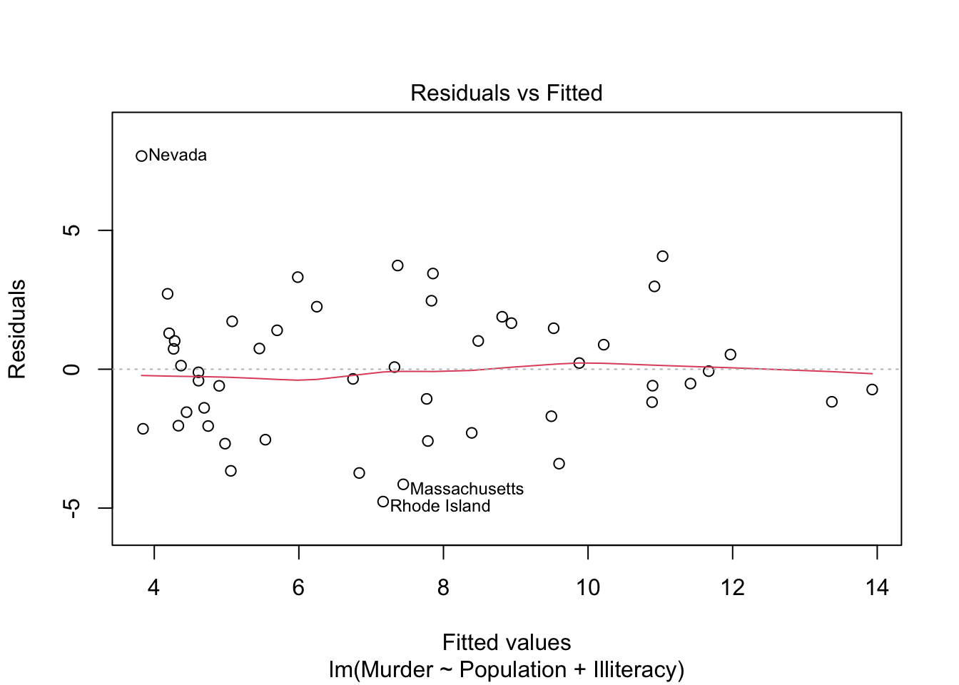
boxTidwell(Murder ~ Population + Illiteracy, data=states) MLE of lambda Score Statistic (t) Pr(>|t|)
Population 0.86939 -0.3228 0.7483
Illiteracy 1.35812 0.6194 0.5388
iterations = 19
Score test for null hypothesis that all lambdas = 1:
F = 0.23214, df = 2 and 45, Pr(>F) = 0.7938If we are dealing with highly skewed data then we might think about applying a log transform. This should also be done if the boxTidwell() output results in a recommendation of 0. Note that you might have to scale or normalize the data as well since you cannot have a log of a negative number.
When the normality assumption is violated then we may want to transform the outcome variable. This could be done as \(Y^\lambda\) with common lambda values as -2, -1, -0.5, 0, 0.5, 1, and 2. To see which type of transformation we should do we can use the powerTransform() function in the car library. If the confidence interval contains the power 1 then we might infer that there is no statistical need to transform the outcome. We have to be careful though, as transforming the outcome will alter the predicted value, thus causing us to have to “reverse” the transformation on the predicted value to see the actual predicted value (if model transformation is \(y^2\) then take the square root to get back to original units).
library(openintro)
model <- lm(mpg_city ~ weight, data=cars93)plot(cars93$weight, cars93$mpg_city)
abline(model, col="red", lwd=2)
plot(model, which=2)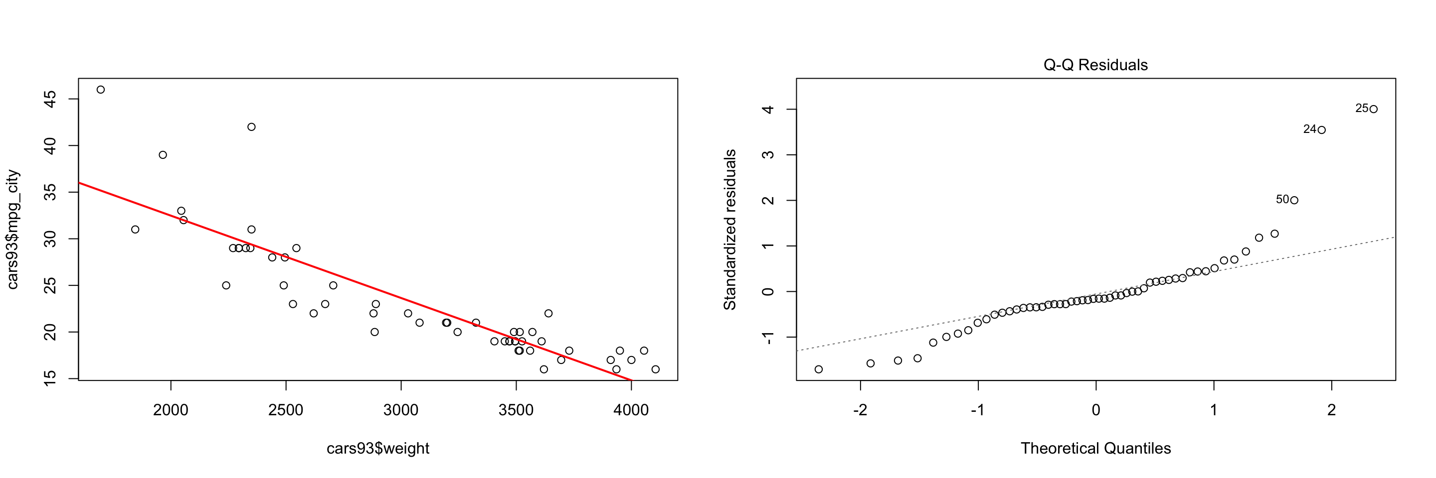
Above we can look at the cars93 dataset in the openintro library to build a model. Looking at the diagnostic plot, we can see that the residuals are not normally distributed. Therefore, we might think that a transformation is needed in order to validate the assumption of normally distributed residuals.
summary(powerTransform(cars93$mpg_city))bcPower Transformation to Normality
Est Power Rounded Pwr Wald Lwr Bnd Wald Upr Bnd
cars93$mpg_city -1.6876 -1 -2.823 -0.5521
Likelihood ratio test that transformation parameter is equal to 0
(log transformation)
LRT df pval
LR test, lambda = (0) 9.477809 1 0.0020797
Likelihood ratio test that no transformation is needed
LRT df pval
LR test, lambda = (1) 25.55596 1 4.2974e-07So, based on these results we can try transforming the outcome variable with an inverse transformation. This will make the model a little harder to interpret, but when we predict values using this model we will just need to make sure to “reverse” the transformation.
model <- lm(I(mpg_city^-1) ~ weight, data=cars93)
summary(model)
Call:
lm(formula = I(mpg_city^-1) ~ weight, data = cars93)

Residuals:
       Min         1Q     Median         3Q        Max
-0.0116148 -0.0014959 -0.0000579  0.0019275  0.0081298

Coefficients:
             Estimate Std. Error t value Pr(>|t|)
(Intercept) 3.670e-04  2.322e-03   0.158    0.875
weight      1.492e-05  7.474e-07  19.959   <2e-16 ***
---
Signif. codes:  0 '***' 0.001 '**' 0.01 '*' 0.05 '.' 0.1 ' ' 1

Residual standard error: 0.003579 on 52 degrees of freedom
Multiple R-squared:  0.8845,    Adjusted R-squared:  0.8823
F-statistic: 398.3 on 1 and 52 DF,  p-value: < 2.2e-16
Looking at the diagnostic plot and a line of best fit, we can see that the residuals look more normally distributed. We can also see that data is fairly linear now (meaning no transformations on the predictors are necessary).
plot(model, which=1)
plot(model, which=2)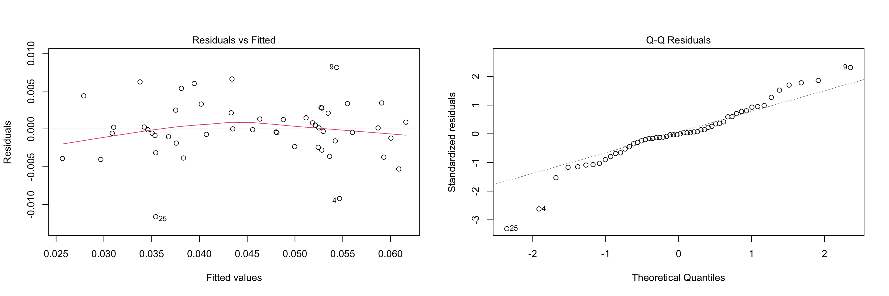
\[\textbf{Model Equation: } \frac{1}{\text{mpg\_city}}= 0.000367 + 0.00001492 \times \text{weight}\]
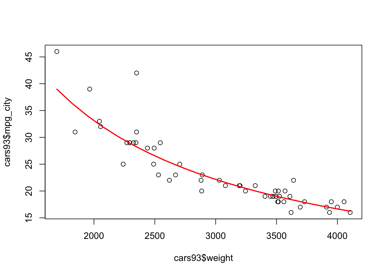
This model tells us that if we have a car that weighs 3,000 units, the city mpg of the car will be 22.16 (found by 1/mpg = 0.045127 and then solving for mpg).
plot(cars93$weight, cars93$mpg_city)
x_values <- seq(min(cars93$weight), max(cars93$weight), length=20)
x_values <- data.frame(weight = x_values)
y_pred <- predict(model, newdata=x_values)
lines(x_values$weight, (y_pred)^-1, col="red", lwd=2)