6 RMarkdown
Switching gears, we are at the point of our Data Science journey where we want to focus on our communication skills so that we can inform others of our findings. To do this we will introduce the idea of reproducibility and a new feature called RMarkdown. Other people need to run our code and reproduce our findings. Because, generating results, no matter how noteworthy, are meaningless if they cannot be independently validated.
- Understand the concept of reproducibility and why it is essential for communicating data results.
- Create an RMarkdown file and recognize its basic components, including the YAML header and R code chunks.
- Write clear narrative explanations outside of code chunks and use them to support understanding of code and output.
- Use the Knit feature to compile an RMarkdown file into a Word or HTML document that combines code, output, and commentary.
Within R there are a few different ways for us to stay organized. One way is to use scripts in R which will allow us to save our code as a .R file and then run the whole file with one command. Another way is to use text documents to save your code as a .txt file, but we cannot run this with a single command. You need to find out what works for you! I normally create my code in the console and then I copy and paste it into a text file when I want to save it. Others open a script and can run it line by line in there, you will just have to play around and create your style. But, when you do code make sure you create it and run it line by line. Very rarely would we want to create multiple lines of code and then run it and “hope” for the best by running it all at once.
6.1 Reproducibility using RMarkdown
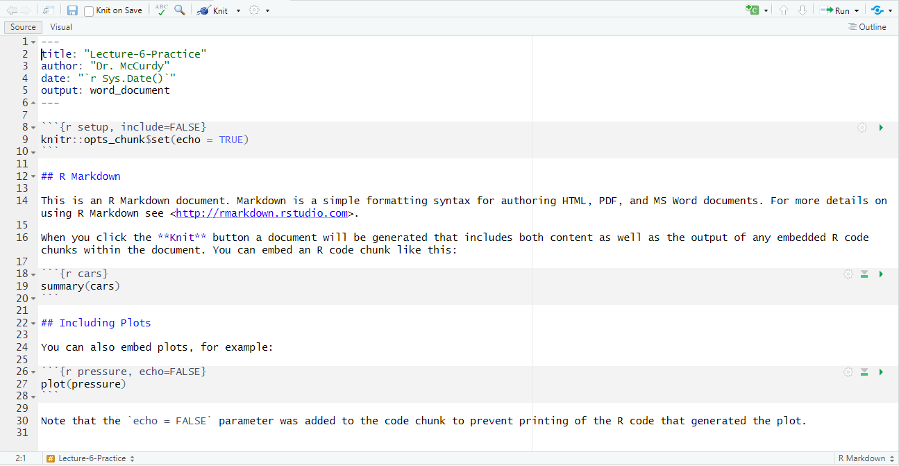
Another system that students tend to like (and one we will be using) is RMarkdown. This is a file type in R that will allow us to place our code comments/explanations, and output side-by-side. We will then be able to “knit” (compile) the file together and it will output a Word document with the output displayed. To access this you will first need to open RStudio, and then you will go to “File -\(>\) New File -\(>\) RMarkdown”. You may need to install some packages on the first run (just accept them). It will then ask you to pick a Title for the document and an output format (just choose Word or HTML, but not choose PDF).
When you create the file, it should look something like this:
6.2 YAML header
RMarkdown relies on YAML (Yet Another Markup Language) so this may be similar to other Markup languages you may have used in other classes. We will just focus on the basics for now, but know that there is a lot of customization and implementations we could do. The Heading will determine the title, output format, and author/date (we will not need to alter anything in here). There are many different ways we can customize the output, but we will keep it fairly simple for now. The YAML header can be seen below, with RStudio updating it automatically for us if we choose different settings.
---
title: "Lecture-6-Practice"
author: "Dr. McCurdy"
date: "`r Sys.Date()`"
output: word_document
---
6.3 R Chunks (where the code goes!)
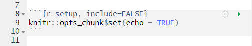
One aspect that we will be adding/altering is the R “Chunks”. These are between the``` symbols and can be created by hitting the green “C” on the top right of the document. These are where we will place the R code (only the code, not the output!) that we want to run. The first chunk of code that is automatically created for us is the setup chunk, which will be run but will not be displayed in the document. This is a good place to load any libraries you are working with or to import different datasets that the reader does not necessarily need to see the details for.
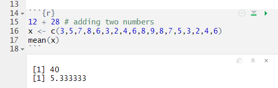
The chunks that we create later on are where we will put our code. We can run the code chunk (and see what the output will look like) by hitting the green play button in the top right portion of the chunk. This will allow us to make sure the code works before we compile the document together. When making our chunk, there are a few different arguments that are available to us, such as echo, eval, include, warning, and message. But, for simplicity, we will ignore all of them for now and just use a chunk with the letter “r” in the curly brackets. In the example chunk below we can see how we are able to run our code in the chunk with the output displayed below it:
6.4 Placing our Explanations
Outside of the R chunks, we will place out explanations of the code/results so others can understand it. To create a “Header”, we can use the pound symbol (#) as long as there is a empty line above and below it with a space between the symbol and the word you want as the header. Using multiple pound symbols will result in smaller sub-headers.
It is possible to emphasize different explanations or words:
- We can italicize words:
*italics* - We can bold words:
**bold** - We can make a bullet-point like by using the - symbol on each line
Additional customization are possible, but we will not go into them right now. Just know that you can click the “Visual” button in the top left-hand corner of the document, and it will alter the file to look more like a “Word” document in terms of buttons to customize the file.
6.5 Knitting the Document
When we are done placing our code and explanations, we will “Knit” it (top middle button) to make it into a Word or HTML document. “Knitting” the document will then compile the file. It will run your R code (or other languages if you specify it) and display the output directly following your code. This results in an organized and professional looking document without having to copy and paste our code/results.
If the document fails to render, it might be because of a few different issues. The first might be that there is a syntax error with our code. It will usually direct you to the “chunk” that broke and tell you what is wrong with it. Another error that we might encounter is a “pandoc” error, which indicates that you currently have the Word document open, and thus is cant compile/overwrite the Word document unless it is closed.