set.seed(12345)
grade_before <- rnorm(100, 80, 5)
grade_after <- grade_before + rnorm(100, 2, 5)15 Comparing Means and Groups
We have seen that we can carry out hypothesis testing on uni-variate variables in order to see if the sample statistic is different (or greater/less than) a certain value. We can expand this idea in order to test if two groups are statistically different from each other as well. The same process will be applied, as we will first need to calculate the point estimate, determine the critical value and standard error, and then determine the test statistic and p-value.
- Distinguish between paired samples and independent samples and choose the appropriate procedure for comparing means.
- Carry out and interpret hypothesis tests for the difference between two population means using paired t-tests and two-sample t-tests.
- Explain when equal-variance and unequal-variance two-sample t-tests are used and how their standard errors differ.
- Use
t.test(),var.test(),aov(), andpairwise.t.test()in R to compare two or more groups and write conclusions in context.
Supplemental Material
15.1 Comparing Two Groups
If we are interested in the difference between two groups then essentially what we are interested in looking at is if the difference between the two is different than 0 (or greater/less than). This gives us a Null Hypothesis of:
\[ H_0: \mu_x=\mu_y \qquad \text{or essentially } \qquad H_0: \mu_x - \mu_y =0 \]
The test statistic can then be found in the usual way:
\[ \text{Test Statistic} = \frac{\text{observed}-\text{hypothesized}}{{SE_{\overline{x}-\overline{y}}}} = \frac{(\overline{x} - \overline{y}) - (\mu_x - \mu_y)}{SE_{\overline{x}-\overline{y}}} \]
The difficult part will be calculating the standard error (\(SE_{\overline{x}-\overline{y}}\)) depending on the scenario. We will look at three cases in this write up. The first is when we have paired data (think before and after) in that every observation from \(x\) is associated with an observation from \(y\). The second is when our data is independent of each other (\(x\) and \(y\) are not connected) and they have equal variance. The third is when our data is independent of each other (\(x\) and \(y\) are not connected) and they have non-equal variance.
15.2 Paired Samples
If the data we wish to compare has some one-to-one relationship then it might be a paired sample (we have to have the same number of observations in each group!). Calculating the standard error is fairly simple as it is just the standard error if the paired difference values. It is common technique to use \(d\) as a subscript to mean the difference.
\[ SE_{\overline{x}-\overline{y}} = s_d/\sqrt{n} \]
Lets look at an example. We want to see if giving someone a piece of chocolate will increase their test scores, so we record their test scores before the chocolate is given and then again after the chocolate is given. We want to see if there is a difference in test scores.
In this case, we are wanting to test:
\[ H_0: \overline{x} - \overline{y}= 0 \qquad \text{vs.} \qquad H_A: \overline{x} - \overline{y} \neq 0 \]
We can look at the point estimator of each group and see if there seems to be a difference or not (but this does not substitute our statistical analysis):
mean(grade_before)[1] 81.22599mean(grade_after)[1] 83.45215grade_diff <- grade_after - grade_before
mean(grade_diff)[1] 2.226166Now, in order to do a paired t-test the differences should follow a normal distribution, and we can confirm this by looking at the qqnorm plot, a histogram, or carrying out a test for normality. I think “eye-balling” it will be good enough for us, but we can do a Shapiro-Wilk Normality Test as well. In this test the null hypothesis will be the values follow a normal distribution and the alternative hypothesis will be that they do not. We can use the shapiro.test() to carry this out:
shapiro.test(grade_diff)
    Shapiro-Wilk normality test

data:  grade_diff
W = 0.98989, p-value = 0.6561
We can see based on this p-value that we will fail to reject the null hypothesis and that we do not have evidence to suggest the values are not normally distributed. So, we are good to go with our paired t-test.
se <- sd(grade_diff)/sqrt(100)
test_stat <- mean(grade_diff)/se
test_stat
[1] 4.40284(1-pt(test_stat, df=99))*2[1] 2.703692e-05Based off this result, we can see that the p-value is small and thus we will reject the null hypothesis. This means we have evidence to suggest that the means are in fact not the same value. Luckily for us, R will carry this calculation out for us, I just wanted to show you that we can still do it ourselves with the exact same process as we did when we previously did hypothesis testing. To do it in R, we can use the t.test() function with the paired argument set to true.
t.test(grade_after, grade_before, paired=TRUE)
    Paired t-test

data:  grade_after and grade_before
t = 4.4028, df = 99, p-value = 2.704e-05
alternative hypothesis: true mean difference is not equal to 0
95 percent confidence interval:
 1.222905 3.229426
sample estimates:
mean difference
       2.226166
Note we can also pass into it a single variable which is the paired-difference between the groups and we get the same result.
t.test(grade_diff)
    One Sample t-test

data:  grade_diff
t = 4.4028, df = 99, p-value = 2.704e-05
alternative hypothesis: true mean is not equal to 0
95 percent confidence interval:
 1.222905 3.229426
sample estimates:
mean of x
 2.226166
15.3 Independent Samples
If our samples are independent of each other then we cannot carry out a paired t-test (which makes sense since our data is not paired…). But, we can still carry out a t-test. If our population standard deviations are known to us then the standard error will simply be:
\[ SE= \sqrt{\text{var}(\overline{x} - \overline{y})} = \sqrt{\sigma^2_x / n_x + \sigma^2_y / n_y} \]
But, we rarely have this information, so we will have to estimate this using the sample standard deviations. And the way we do it will depend on whether or not our samples have an equal or unequal variance.
If the samples have equal variances then the standard error can be calculated by:
\[ SE_{\overline{x} - \overline{y}} = \sqrt{s_p^2 \left(\frac{1}{n_x} + \frac{1}{n_y} \right)} \] where \(s_p\) is the pooled variance. This will give us a better standard deviation estimator since we assume the variance is the same and it is better to have ``more values” in order to be more accurate. This can be calculated as:
\[ s_p^2 = \frac{(n_x - 1)s_x^2 + (n_y-1)s^2_y}{n_x + n_y - 2} \]
where the \(df=n_x + n_y - 2\) since we are estimating two values (\(s_x\) and \(s_y\)).
Once we have calculated the standard error then the process is the exact same as all of our other hypothesis testing. Below we can see an example of this using simulated data:
set.seed(123)
x <- rnorm(30, 11, 2)
y <- rnorm(35, 10.5, 2)
mean(x)
[1] 10.90579mean(y)[1] 10.66022We will first want to see if the samples have an equal variance. We will use the var.test() function to do this which has a null hypothesis of equal variance and an alternative hypothesis of unequal variance. This test will rely on an F-test (along with an F-distribution), but that is not vital for us to understand. We are interested in is if the variances are equal or not.
var.test(x, y)
    F test to compare two variances

data:  x and y
F = 1.3837, num df = 29, denom df = 34, p-value = 0.3614
alternative hypothesis: true ratio of variances is not equal to 1
95 percent confidence interval:
 0.6847548 2.8534854
sample estimates:
ratio of variances
          1.383669
This indicated that we have equal variance (which is good since the simulation had equal variances). Because we have this we can continue with our calculations:
n_x <- length(x)
n_y <- length(y)
var_x <- var(x)
var_y <- var(y)
pooled_var <- ((n_x - 1)*var_x + (n_y-1)*var_y)/(n_x + n_y - 2)
pooled_var
[1] 3.273598se <- sqrt(pooled_var* (1/n_x + 1/n_y))
se[1] 0.4501681test_stat <- (mean(x) - mean(y))/se
test_stat[1] 0.5455076(1-pt(test_stat, df=n_x + n_y - 2))*2[1] 0.5873308Based on this result, we can see that we will fail to reject the null hypothesis, meaning that we do not have evidence to suggest the mean of the two groups are difference from each other. Luckily, we can do this in R as well and we get the exact same result:
t.test(x, y, var.equal = TRUE, paired=FALSE)
    Two Sample t-test

data:  x and y
t = 0.54551, df = 63, p-value = 0.5873
alternative hypothesis: true difference in means is not equal to 0
95 percent confidence interval:
 -0.654019  1.145159
sample estimates:
mean of x mean of y
 10.90579  10.66022
Now, if we were to determine that the variances were not equal to each other then we have to approach the problem a little bit differently. In this case the the standard error and the degrees of freedom can be found below:
\[ SE_{\overline{x} - \overline{y}} = \sqrt{\frac{s_x^2}{n_x} + \frac{s_y^2}{n_y}} \]
\[ df= \left( \frac{s_x^2}{n_x} + \frac{s_y^2}{n_y}\right)^2 \cdot \left( \frac{\left(\frac{s_x^2}{n_x} \right)^2}{n_x -1}+ \frac{\left(\frac{s_y^2}{n_y} \right)^2}{n_y -1} \right)^{-1} \]
We do not want to calculate this in R manually, but we can see an example of this below with simulated data:
set.seed(123)
x <- rnorm(30, 11, 2)
y <- rnorm(35, 10.5, 7)
var.test(x,y)
    F test to compare two variances

data:  x and y
F = 0.11295, num df = 29, denom df = 34, p-value = 5.188e-08
alternative hypothesis: true ratio of variances is not equal to 1
95 percent confidence interval:
 0.05589835 0.23293758
sample estimates:
ratio of variances
         0.1129526
The variance test indicates that the variances are not equal to each other. Therefore, we cannot use the exact same set-up as we did in the previous problem. Instead we have to use the formulas directly above in order to calculate the standard error and the degrees of freedom. Note that in this method the degrees of freedom may end up being a non-integer (but the interpretation of this is beyond our scope).
n_x <- length(x)
n_y <- length(y)
var_x <- var(x)
var_y <- var(y)
se <- sqrt(var_x/n_x + var_y/n_y)
se
[1] 1.049811df <- (var_x/n_x + var_y/n_y)^2 * ((var_x/n_x)^2/(n_x -1) +
(var_y/n_y)^2/(n_y-1))^-1
df[1] 42.68234test_stat <- (mean(x)-mean(y))/se
test_stat[1] -0.1476322(pt(test_stat, df=df))*2[1] 0.8833282Based on this we can see the p-value is larger than our significance level (0.05) so we will fail to reject the null hypothesis and conclude the groups have the same mean. We do not want to have to calculate everything like this in R every time, we can use the function to do it for us. Notice that we get the exact same result.
t.test(x, y, var.equal = FALSE, paired=FALSE)
    Welch Two Sample t-test

data:  x and y
t = -0.14763, df = 42.682, p-value = 0.8833
alternative hypothesis: true difference in means is not equal to 0
95 percent confidence interval:
 -2.272587  1.962615
sample estimates:
mean of x mean of y
 10.90579  11.06078
Everything we have done so far has been written as a two-sided test. You can change the alternative hypothesis to a one-sided test if you wish. The process will be the exact same, the only difference will be in calculating the p-value. This was shown in a previous lecture.
15.4 Comparing Multiple Groups
If instead of just two groups we are dealing with multiple groups then we have to approach the problem a little bit differently. The reason is because when we run a t-test, we have an \(\alpha\) risk of a Type I error occurring (normally 0.05). If we were to run multiple t-tests across groupings then this increases the risks of making a Type I error. To get around this issue, we will introduce One-way ANOVA (Analysis of Variance). This will allow us to determine if there is a significant difference across any level of categorical variables. We should note that this does not tell us which levels are statistically different, it only tells us that at least one group mean differs.
\[ H_0: \mu_1 = \mu_2 = \dots = \mu_k \qquad \text{vs.} \qquad H_A: \text{not all group means are} \]
It we determine that at least 2 are different then each other, then we can run pairwise t-tests in order to see which ones are different.
To run an ANOVA model in R, we will use the aov() function. With this function we have to pass it in a “formula” we want evaluated. For us it will be “Quant Vector ~ Qual Group”. We will also need to save the output to a variable and then view a summary of it in order to see the p-value.
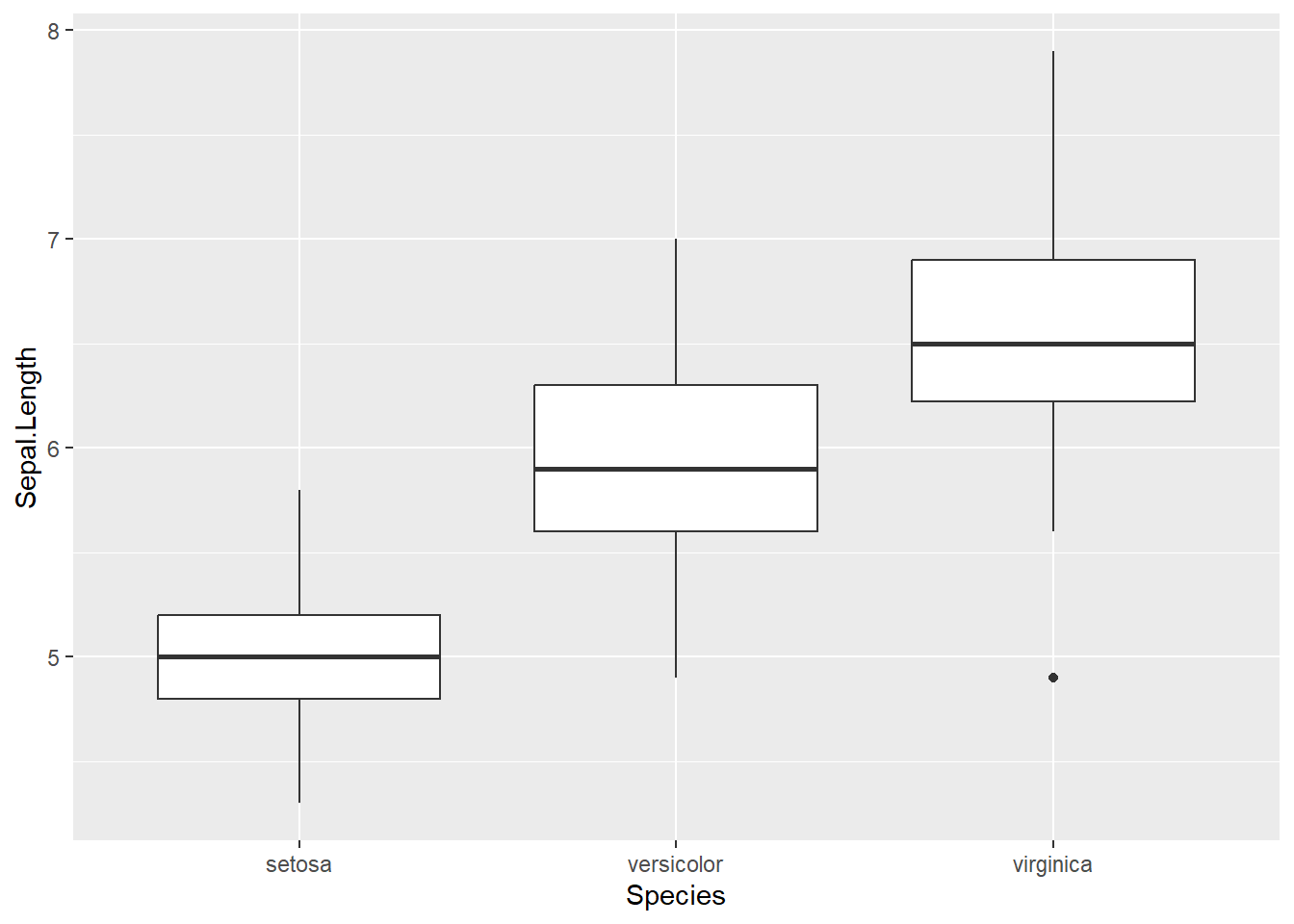
In the example below, I am interested in seeing if there is a difference in Sepal Length for different iris Species. We can create a boxplot and see that it does appear there is a difference in the sepal length for each species. But, we will need to carry out an ANOVA model to see if this is actually true.
anova_model <- aov(Sepal.Length ~ Species, data=iris)
summary(anova_model)
Df Sum Sq Mean Sq F value Pr(>F)
Species 2 63.21 31.606 119.3 <2e-16 ***
Residuals 147 38.96 0.265
---
Signif. codes: 0 '***' 0.001 '**' 0.01 '*' 0.05 '.' 0.1 ' ' 1Since the p-value for the species is very small, we will reject the null hypothesis and claim that there is a difference between at least two groups in the data.
Now that we have made this determination, we can carry out a pairwise t-test to see where there is a difference between groups. To do this we use the pairwise.t.test() function with a p-adj="bonferroni". This will adjust the p-values slightly since we have multiple groups.
pairwise.t.test(iris$Sepal.Length, iris$Species, p.adj = "bonferroni")
    Pairwise comparisons using t tests with pooled SD

data:  iris$Sepal.Length and iris$Species

           setosa  versicolor
versicolor 2.6e-15 -
virginica  < 2e-16 8.3e-09

P value adjustment method: bonferroni
With this output, we can see that every group is actually different from each other. Lets look at a different example with simulated data:
set.seed(123)
v <- rnorm(100, 10, 2)
w <- rnorm(100, 11, 2)
x <- rnorm(100, 12, 2)
y <- rnorm(100, 13, 2)
z <- rnorm(100, 14, 2)

example_prob <- data.frame(value=c(v, w, x, y, z),
                           category=rep(c("V", "W", "X", "Y", "Z"), each=100))
We will first run an ANOVA model. This shows us there is a difference it at least two groups. When we do a pairwise t-test we can see that some categories are statistically different then others, but are not.
anova_model <- aov(value~category, data=example_prob)
summary(anova_model)
Df Sum Sq Mean Sq F value Pr(>F)
category 4 1057 264.30 69.87 <2e-16 ***
Residuals 495 1872 3.78
---
Signif. codes: 0 '***' 0.001 '**' 0.01 '*' 0.05 '.' 0.1 ' ' 1pairwise.t.test(example_prob$value, example_prob$category, p.adj="bonferroni")
    Pairwise comparisons using t tests with pooled SD

data:  example_prob$value and example_prob$category

  V       W       X       Y
W 0.29    -       -       -
X 3.2e-12 1.8e-06 -       -
Y < 2e-16 4.0e-13 0.13    -
Z < 2e-16 < 2e-16 2.8e-11 3.9e-05

P value adjustment method: bonferroni
Let us look at one final example to see this in action. This example is to show us that we should be careful with what we are doing. We will only do a pairwise t-test if ANOVA tells us that at least two groups are statistically different. In this case, the ANOVA tells us that the model is slightly significant (the p-value is pretty close to 0.05). Typically we would fail to reject the null and conclude that there is not a statistical difference between groups. But, if we were to do a pairwise t-test we would see a difference.
set.seed(123)
w <- rnorm(100, 11.6, 3)
x <- rnorm(100, 10, 2)
y <- rnorm(100, 10, 5)
z <- rnorm(100, 11, 9)
df <- data.frame(values=c(w,x,y,z),
                 type=rep(c("W", "X", "Y", "Z"), each=100))

anova_model <- aov(values~type, data=df)
summary(anova_model)
Df Sum Sq Mean Sq F value Pr(>F)
type 3 221 73.83 2.437 0.0643 .
Residuals 396 11999 30.30
---
Signif. codes: 0 '***' 0.001 '**' 0.01 '*' 0.05 '.' 0.1 ' ' 1